D1 · Publication Volume 17
Implicit Geological Modelling
scalar fields, interpolation, trends and parameters
Learning objectives
By the end of this lesson, the learner should be able to describe a geological surface as a level set of a scalar field; distinguish contact, orientation and inequality constraints; explain how interpolation, trend, anisotropy, support and resolution affect geometry; compare parameterisations without treating an automatically generated surface as objective; and validate an implicit result against both data and geological relationships.
Implicit modelling replaces direct drawing of every triangle with an estimated field. A surface is extracted where the field reaches a chosen value. The method can update consistently when constraints change and can represent several conformable contacts in one field, but its output still depends on interpretation, parameter choices and geological rules.
Scalar fields and level sets
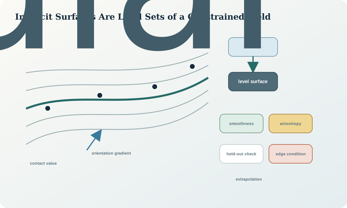
Let f(\mathbf{x}) be a scalar value defined throughout the model volume. A geological surface S_c is the set of locations where
S_c=\{\mathbf{x}:f(\mathbf{x})=c\}.
For a stratigraphic package, different values c_1,c_2,\ldots may represent ordered contacts. The numerical field is not necessarily age, elevation or distance; it is a coordinate-like device whose ordering and gradient encode geological structure. Its meaning must be stated. Treating arbitrary field values as physical measurements creates false interpretation.
The gradient \nabla f(\mathbf{x}) is normal to a level surface. Orientation data can therefore constrain gradient direction. Contact points constrain field value. Relative-order or inequality constraints may specify that a location lies above, below or inside a unit without forcing an exact boundary position.
Constraint types and weighting
Separate direct contact points, derived contacts, orientation measurements, interpreted guides and boundary conditions. Give each a quality state and uncertainty. Weight is not a substitute for meaning: doubling a duplicated point must not make one observation twice as true. Detect clustered or repeated constraints before assigning numerical influence.
Orientation constraints can dominate sparse areas. Check polarity, angular uncertainty and structural domain before combining them. A regional trend may help stabilise interpolation, but it should be an explicit prior or guide, not hidden inside default parameters. Hold back some observations when density permits so that validation is not entirely circular.
Interpolation, smoothness and anisotropy
Implicit methods choose a field that balances data fit with smoothness or another regularisation criterion. Strong smoothness can suppress real folds, pinches or angular contacts. Weak regularisation can produce oscillation around noisy constraints. Anisotropy changes the directions over which information propagates; it should follow geological structure or a tested hypothesis rather than screen appearance.
Parameter names differ among implementations, but the audit questions remain stable: What objective is minimised? How are contact and gradient residuals scaled? What is the neighbourhood or basis support? How are discontinuities handled? What boundary conditions act at model edges? Which parameters materially change the interpreted geometry?
Multiple horizons, unconformities and intrusions
Conformable horizons can share one field when their ordering and structural geometry are compatible. Unconformities require truncation rules between packages. Intrusions and other non-stratigraphic bodies may need separate fields or inside–outside constraints. Forcing all objects into one stratigraphic field can create impossible order or unintended connections.
State the relationship graph before evaluation. A younger erosion surface truncates older units; a later intrusion cuts both; a fault may displace all earlier features. The scalar fields provide geometry, while the relationship graph provides geological assembly. Neither is sufficient alone.
Resolution, extraction and numerical effects
The field may be solved or evaluated on a grid, mesh or basis with finite resolution. The extracted isosurface depends on evaluation spacing and contouring algorithm. A thin unit can vanish if the sampling step exceeds its field separation. Two surfaces can appear to touch or cross because of extraction resolution even when the continuous fields remain ordered.
Perform refinement tests. Evaluate the same field on progressively finer supports and compare contact positions, topology, volumes and minimum thickness. If results change materially, report the numerical sensitivity. Dense evaluation cannot recover a feature absent from the constraints or geological formulation.
Synthetic worked example
The fictional folded horizon has eighteen contact points and nine orientations. A first implicit field uses all orientations equally and a strong regional trend. It honours contact points but straightens the northern fold limb and predicts an unsupported deep continuation. A second run removes two low-confidence orientations, restricts the trend to the southern domain and reduces smoothness near the hinge.
Comparison uses held-out contacts, curvature, minimum thickness, distance-to-data and intersection with the fault framework. The second field better predicts held-out points, but both remain plausible below the deepest hole. That deep difference is retained as scenario uncertainty rather than resolved by choosing the smoother image.
Practice and review checklist
Fit or conceptually compare at least three implicit parameter sets. Change one material assumption at a time and record:
- contact and orientation residuals by quality class;
- held-out prediction where possible;
- surface curvature and minimum feature thickness;
- model-edge behaviour;
- topology and volume changes;
- distance from each surface region to direct constraints; and
- whether a parameter change expresses geology, numerical stability or visual preference.
Reject any run that fits numeric residuals while violating required geological order or topology.
Decision implications and integration
Release the field definition, constraint version, parameter set, solver or algorithm version, extraction resolution and resulting surface identifiers together. If only the mesh is preserved, the implicit model cannot be reproduced or updated reliably.
Pass both the surfaces and the relationship graph to fault, solid and domain construction. Mark regions whose geometry is controlled primarily by priors, boundary conditions or extrapolation so downstream users do not mistake interpolation coverage for evidence coverage.
Sources
- LoopStructural 1.0, explains scalar fields, gradients, structural frames and geological feature interactions.
- GemPy 1.0, describes implicit potential-field interpolation and stochastic structural modelling.
- Building 3D geological models directly from the data, discusses potential-field construction and updating from geological observations.
- Three-dimensional geologic maps and visualization, relates constrained surfaces, uncertainty and interaction rules.