C3 · Publication Volume 13
The Geochemical Exploration Signal Chain
source, dispersion, sampling, analysis and interpretation
Learning goals
This lesson establishes the causal model used in every later chapter. The learner should be able to trace a reported concentration backward through analysis, preparation, collection, medium and dispersion to a geological source; identify where amplitude, location or composition can change; distinguish a source signal from an observation-process artefact; and specify a test that isolates a weak link.
The central discipline is to avoid the shortcut “high value equals nearby source.” A high value may reflect a concentrated resistant mineral, a narrow sample support, evaporation, adsorption, external material, incomplete mixing, contamination or a unit error. A modest value may be important where dilution, cover or partial extraction attenuates a coherent process signal. Interpretation begins with the chain, not with colour classes.
Geological source and element residence
A source is a spatial distribution of elements in minerals, fluids, glass, organic matter or adsorbed phases. Bulk concentration alone is insufficient. Residence determines liberation, grain size, density, reactivity and response to extraction. An element held in a resistant accessory grain may travel mechanically and survive strong weathering. The same element adsorbed to an oxide coating may be mobile across changing acidity or redox conditions and recoverable by a weak extraction.
Define the source hypothesis at an observable scale. “Mineralisation exists” is too broad. A useful statement identifies the process, host material, expected carriers, approximate geometry, alteration or weathering relation, and elements predicted to be enriched or depleted. It also names an alternative source such as ordinary lithological variation or externally introduced material.
Source heterogeneity creates sampling variance. A few coarse grains can dominate a small aliquot even when the bulk medium is only weakly enriched. This is not merely instrument noise. It is a mismatch between particle distribution, collected mass, split mass and analytical portion. Mineralogical examination and staged mass checks may be more informative than repeating the same tiny aliquot.
Primary dispersion from geological processes
Primary dispersion forms during or soon after the geological process of interest. Fluid flow can alter wall rock, exchange elements and form zoned mineral assemblages. Magmatic differentiation can partition elements among melt and minerals. Metamorphic reactions can mobilise or immobilise components. Mechanical emplacement can distribute fragments along structures. These footprints may extend beyond the high-concentration source but remain controlled by permeability, reaction, temperature, host composition and time.
Translate the process into a predicted vector rather than a list of “pathfinder” elements. State which element or ratio should increase, which should decrease, which mineral or phase carries it, how far the effect could extend, and which competing process produces a similar signature. A footprint is useful only when the observation method can detect it at its actual support and depth.
Primary signatures are commonly overprinted. Later alteration can add, remove or redistribute the same elements. Weathering can destroy carrier minerals. Mixing can blur zoning. Therefore, absence in a surface medium is negative evidence only when preservation, exposure, support and analytical sensitivity were adequate.
Secondary dispersion and observation footprint
Secondary dispersion begins when weathering and surface processes transform or transport source material. Mechanical dispersion moves particles downslope or downstream. Chemical dispersion involves dissolution, complexing, adsorption, precipitation and exchange. Hydromorphic pathways integrate water movement and seasonal conditions. Biological uptake selectively samples accessible forms over a root or tissue support. Human activity can introduce or redistribute material unrelated to geology.
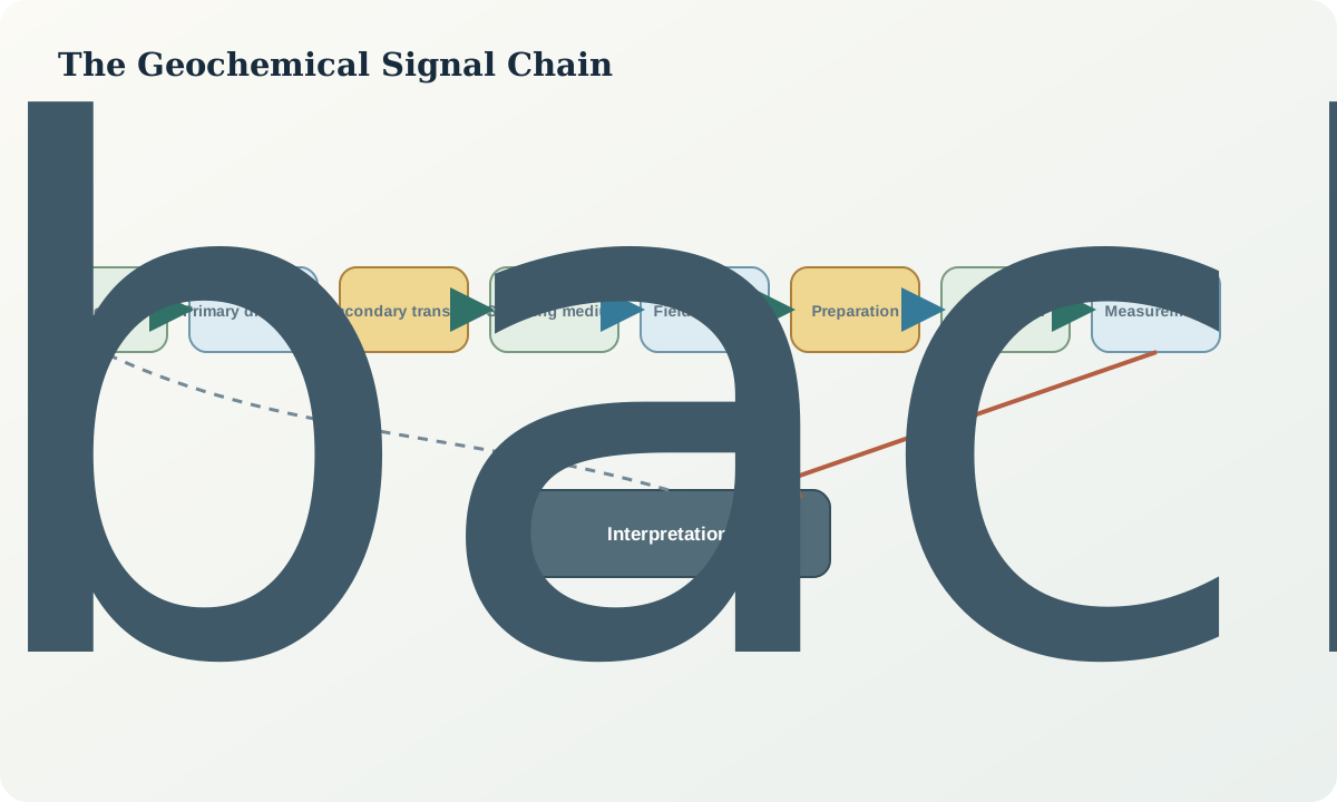
The observation footprint is the area, depth and time represented by a sample. A drainage sediment sample may integrate an upstream catchment but disproportionately represent erodible units, fine fractions, depositional traps and recent flows. A soil sample integrates a small volume yet may contain transported cover. Water may respond quickly to flow state and preservation. Rock chips may closely locate bedrock but under-represent concealed or weakly exposed material.
Record directionality. A displaced signal should not be plotted as though its source lies at the sample point. The sample coordinate identifies collection; the inferred source area is a separate geometry with an uncertainty envelope. Transport distance is a hypothesis to test using grain character, terrain, catchments, horizons and multi-medium observations.
Sampling, preparation and measurement transfer
At collection, the target population becomes a finite physical increment. At preparation, that increment is dried, screened, crushed, milled, split or otherwise reduced. At extraction, only an operationally defined fraction may enter solution. At measurement, calibration and interference controls convert response into a reported value. Each transfer has a recovery, selectivity and contamination risk.
A practical transfer model is
$y = C_s f_l f_m f_r + c + \epsilon,$
where C_s is source-scale concentration, f_l is liberation and dispersion retention, f_m is the fraction represented by the chosen medium and support, f_r is preparation-and-extraction recovery, c is introduced contamination and \epsilon combines random components. The factors are not assumed independent or constant. The equation is a checklist: a result can change because the source changed, because a transfer factor changed, or because contamination or noise changed.
Quality controls must be placed at the stage they diagnose. A laboratory blank cannot reveal contamination introduced by a field tool before the sample arrived. A field duplicate contains field heterogeneity plus later variation; an analytical repeat isolates a much narrower portion of the chain. Comparing them helps locate the dominant uncertainty.
Worked synthetic example
A synthetic source material contains 1,200 mg/kg of element X. A simplified model assumes 0.60 of the source signal is liberated into the sampled surface pathway, 0.50 remains in the selected size fraction, the collected support represents 0.80 of that fraction and preparation plus extraction recovers 0.90. No contamination is assumed. The expected result is
$1{,}200(0.60)(0.50)(0.80)(0.90)=259.2\ \mathrm{mg/kg}.$
If domain background is 40 mg/kg, the expected contrast is 259.2/40=6.48. Now suppose the wrong coarse fraction is selected and retains only 0.10 rather than 0.50. The expected value becomes 51.84 mg/kg, only 1.30 times background. A non-anomalous classification would not refute the source hypothesis; it would show that the chosen transfer path had poor sensitivity.
Alternatively, a 25 mg/kg contamination contribution produces 284.2 mg/kg in the first design and 76.84 mg/kg in the poor-fraction design. The contamination is a small relative effect on the strong signal but can create a false anomaly in the weak one. A blank inserted after field collection would miss contamination from the sampling tool. The example shows why amplitude and diagnostic controls must be interpreted together.
Signal-chain audit workflow
- State the geological process and alternative sources.
- Identify carrier phases and predicted enrichment, depletion or ratio changes.
- Map primary and secondary dispersion pathways with direction and scale.
- Define the medium's spatial, depth, particle and temporal support.
- Record field selection, tools, containers, preservation and custody.
- Trace every preparation, split, extraction, dilution and measurement step.
- Place controls beside the failure mode they can detect.
- Preserve limits, qualifiers, units, method codes and batch identities.
- Compare observed patterns with source, transport and artefact hypotheses.
- Design the next observation to separate the most consequential alternatives.
Practice and review
- Draw two signal chains for the same concealed source: one using residual soil and one using stream sediment. Mark where the source location could be displaced.
- Recalculate the synthetic example with liberation 0.35 and recovery 0.75. Explain whether additional instrument precision would repair the loss of contrast.
- List three ways a high concentration can arise without a high local bedrock concentration.
- Match a field blank, field duplicate, preparation duplicate and analytical repeat to the chain segment each can diagnose.
- Write a negative-result rule that distinguishes “source unlikely” from “test insensitive.”
Review questions: What physical material does the number represent? Which factors can attenuate or add signal? Where is the inferred source relative to the sample? Which control can detect the suspected failure? What observation would change the interpretation?
Sources and further reading
- Principles of geochemical prospecting, presents foundational relationships among source, dispersion and sampling.
- Geochemical exploration media overview, reviews media and process controls on observable signals.
- Regolith and geochemical mapping concepts, connects surface materials, mapping and interpretation.
- Uncertainty arising from sampling, separates sampling and analytical contributions to measurement uncertainty.