C3 · Publication Volume 13
Background, Threshold and Anomaly
populations, robust statistics and spatial context
Learning goals
The learner should be able to define background as a process- and domain-dependent population rather than one global constant; distinguish a statistical threshold from a geological boundary; use robust summaries without assuming they reveal a unique population; preserve spatial context and sampling support; and treat an anomaly as an observation to explain with source, transport, lithology, environment and artefact hypotheses.
Anomaly is relational. A value may be unusual for one lithology, horizon, catchment size or analytical method and ordinary for another. A threshold can help prioritise review, but it cannot decide geological origin. Domain construction and observation quality precede threshold calculation.
Background populations and domains
Background includes natural variation produced by ordinary geological and surface processes for the question at hand. It is rarely a single normal distribution. Lithology, weathering, grain size, organic content, drainage area, salinity, landform, method and censoring can create overlapping populations. External material can add another population.
Define domains using variables available independently of the target result where possible. If domains are drawn around high values after viewing them, the estimated background is circular. Record domain evidence, scale and uncertainty. Small domains with few samples may require partial pooling or wide bounds rather than unstable local thresholds.
Background is not synonymous with barren. A mineralised system can contribute to a regional baseline, and unmineralised lithology can be naturally enriched. A global crustal average does not replace local, support-matched observations. Compare like medium, fraction, method and process domain.
Robust summaries and threshold choices
The median and median absolute deviation resist a limited number of extreme values, but they do not automatically separate populations. Quantiles provide empirical ranks but depend on sample design. Transformations can stabilise multiplicative variation. Mixture, spatial and regression models may adjust for covariates, but their assumptions and uncertainty must be checked.
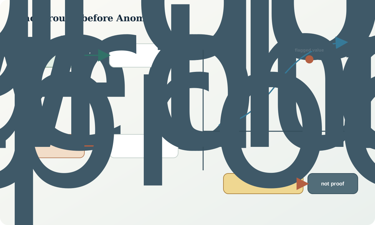
A threshold may be percentile-based, robust-location based, model-residual based, decision-theoretic or tied to orientation evidence. Each answers a different question. “Top 2%” guarantees flags even in a background-only population. A robust cutoff can miss a broad low-contrast footprint. A supervised cutoff can overfit known targets. Report the rule and sensitivity across defensible alternatives.
Use multiple levels where useful: detection concern, review threshold, coherent anomaly and action threshold. Do not imply false numeric precision. Near-boundary samples should be interpreted with uncertainty, neighbours, controls and process evidence rather than classified as fundamentally different.
Spatial and multivariate context
An isolated high value may be a rare grain, transcription error, contamination or a real narrow source. Coherence across adjacent support-matched samples, multiple media or process-related elements increases interpretability, but spatial autocorrelation means neighbouring evidence is not independent. A broad trend can reflect lithology or transport rather than a target process.
For multivariate background, element associations and ratios may distinguish processes that single-element amplitude cannot. However, closed compositions, censoring and shared denominators can create spurious structure. Establish univariate data quality and domains first. Use mineralogical or field evidence to connect the statistical pattern to a carrier and mechanism.
Map sampling density, limits, method, domain and quality status alongside concentrations. An apparent anomaly edge may be a method boundary. An apparent low may be censored. Interpolation across unsampled domain boundaries can manufacture continuity. Keep observed points visible.
From statistical flag to geological anomaly
A geological anomaly has a defensible contrast, coherent support, adequate quality and a plausible process link. Review source and carrier, dispersion direction, medium sensitivity, controls, repeatability, spatial continuity, element association and negative evidence. Build at least one ordinary-lithology, transport or artefact alternative.
Threshold exceedance is not required for every useful signal. A subtle but coherent ratio or depletion zone may be predicted. Conversely, a very high value can be irrelevant to the intended source if its carrier is external or detrital. The interpretation should predict a follow-up pattern, not merely restate the observed high.
Record anomaly geometry separately from target geometry. The anomaly is an observation footprint; the target is an inferred source or process region. Their displacement and uncertainty are central to follow-up design.
Worked synthetic example
A synthetic support-matched domain has X values 12, 14, 15, 16, 16, 17, 18, 20, 22 and 65 mg/kg. The median is (16+17)/2=16.5. Absolute deviations are 4.5, 2.5, 1.5, 0.5, 0.5, 0.5, 1.5, 3.5, 5.5 and 48.5; their median is (1.5+2.5)/2=2.0 mg/kg.
Using a scaled deviation 1.4826(2.0)=2.9652 and an illustrative review rule of median plus three scaled deviations gives
$T=16.5+3(2.9652)=25.40\ \mathrm{mg/kg}.$
Only 65 exceeds the rule. This does not prove a separate geological population. If the 65 mg/kg sample is a preparation blank, it indicates contamination; if it is a coarse lag sample among fine soil samples, support differs; if it lies within a coherent process footprint and controls pass, it becomes a follow-up anomaly.
If a second defensible domain includes naturally enriched lithology with median 55 mg/kg, the same value of 65 may be ordinary. A global 25.40 mg/kg threshold would over-flag that lithology. Domain choice is more consequential than decimal precision in the formula.
Threshold audit workflow
- Confirm identity, units, methods, limits, controls and support.
- Define geological and surface-process domains independently of the anomaly where possible.
- Profile censoring, skew, mixtures, spatial density and batch structure.
- Summarise each domain with robust centre, spread and empirical ranks.
- Choose threshold rules tied to review or action, not visual convention.
- Test sensitivity to domain boundaries and plausible statistical rules.
- Map observations, sampling coverage, limits and quality status together.
- Evaluate carrier, dispersion, lithology, transport and artefact hypotheses.
- Separate observation anomaly geometry from inferred target geometry.
- Design follow-up that predicts contrasting outcomes among hypotheses.
Practice and review
- Recalculate the synthetic threshold after removing 65 and explain why removal must be justified independently.
- Construct two process domains where the same 40 mg/kg result has different meanings.
- Explain why a 98th-percentile rule always creates “anomalies” in a background-only dataset.
- Design a map legend that distinguishes censored, failed, unsampled and quantified low observations.
- Write three competing explanations for a single extreme stream-sediment value.
Review questions: Which population defines background? Is the threshold tied to a decision? Are supports and methods comparable? Is the pattern coherent and quality-controlled? What mechanism predicts the next observation?
Sources and further reading
- Robust multivariate adjustment of geochemical background, shows why background can require covariate-aware robust treatment.
- Statistical identification of geochemical thresholds90002-8), presents a foundational threshold framework and its assumptions.
- Characterising background and anomalous populations90085-9), examines separation of geochemical populations.
- Probability-based threshold interpretation90030-2), connects probability models with threshold decisions.