C4 · Publication Volume 14
From Rock Properties to Geophysical Response
property contrast, geometry, depth, noise and survey configuration
Learning goals
This lesson establishes the physical language for all later methods. The learner should be able to replace a rock-name expectation with a property-contrast hypothesis; distinguish intrinsic property from effective survey response; predict how geometry and distance change amplitude and wavelength; identify the support of a measurement; and design a simple forward test before interpreting an anomaly.
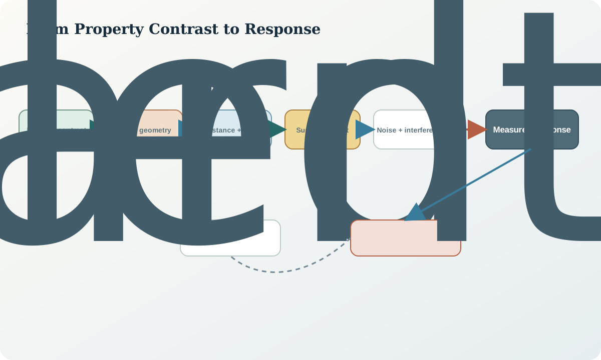
The essential correction to intuition is that instruments do not identify lithology. They measure fields, potentials, count rates, voltages, accelerations, arrival times or derived quantities. A material becomes detectable only when its relevant property differs from its surroundings, occupies sufficient volume, lies within the sensitivity footprint and produces a signal distinguishable from acquisition and environmental variability.
Property contrast, not material label
Density, magnetic susceptibility, remanent magnetisation, electrical conductivity, chargeability, dielectric response, radioelement abundance, seismic velocity and attenuation are physical properties or effective parameters. None maps one-to-one onto a geological name. The same rock type can span a wide property range because of mineral proportions, porosity, fluid, temperature, fabric, alteration and weathering. Different rocks can share the same effective property.
Define contrast relative to a host or reference domain. If a body and host have densities \rho_b and \rho_h, the gravity-relevant contrast is \Delta\rho=\rho_b-\rho_h. If their conductivities are equal, an electrical method has no contrast to detect even if the geological contact is important. A gradual property transition produces a different response from a sharp boundary with the same end-member values.
Property values must have measurement conditions. Direction matters for anisotropic materials. Electrical response can depend on frequency; induced polarisation on time window; seismic velocity on propagation direction and pressure; magnetic response on applied field and remanence; radiometric response on surface state and moisture. A laboratory plug and an in situ volume do not necessarily have equivalent support or condition.
Geometry, depth and distance
Response depends on where property contrast is located and how it is shaped. Volume, thickness, dip, strike length, top depth and boundary roughness can trade off against property magnitude. A small strong body may resemble a larger weak one. A deep compact source tends to produce a broader, lower-amplitude surface response than an otherwise similar shallow source. These are general sensitivity relations, not unique depth rules.
Potential-field influence is spatially broad and commonly decays rapidly with distance. Wave and diffusion methods add source–receiver geometry, propagation path and bandwidth. Borehole tools sample a local volume around a trajectory. Radiometric measurements are dominated by a shallow surface layer and attenuated by air, water and cover. The word “depth” therefore has method-specific meanings: top of a model body, sensitivity centroid, investigation depth, skin depth, penetration, first arrival path or tool radius.
Always draw geometry in a declared coordinate frame. Include the measurement position, sensor height or depth, source and receiver orientation, property body and host, terrain or borehole path, and any air or cover layer. A plan-view anomaly cannot establish dip without directional or depth information.
Forward response and sensitivity
A forward model computes observations from a proposed property distribution and acquisition geometry. In compact notation, \mathbf d^{\mathrm{pred}}=F(\mathbf m,\mathbf g). The operator may be an analytic formula, numerical integration, finite-volume or finite-element solution, ray calculation or convolution. Its purpose is not merely to make a realistic image. It tests whether the proposed model can produce the observed sign, amplitude, wavelength, direction and bandwidth under stated physics.
Sensitivity asks how much an observation changes when a model parameter changes. For a small perturbation, \Delta\mathbf d\approx J\Delta\mathbf m, where J is a sensitivity matrix. Large sensitivity does not guarantee uniqueness: two columns of J may be similar, allowing parameters to trade off. Low sensitivity means a parameter is weakly constrained regardless of a smooth-looking model.
Run scale tests before detailed inversion. Change one factor at a time: halve contrast, double depth, narrow width, rotate strike, raise the sensor, increase cover conductivity or remove a component. Plot the difference in data space, not only model space. If the difference is smaller than realistic uncertainty, the survey cannot discriminate those alternatives.
Noise, interference and measurement support
Noise includes random instrument variation, timing error, navigation error, platform motion, environmental change and poorly modelled background. Interference is structured signal from sources outside the intended geological hypothesis: infrastructure, topography, near-surface heterogeneity, other geological bodies or processing artefacts. Calling all unexplained variation “noise” hides potentially diagnosable processes.
Measurement support is the spatial, temporal and directional volume that contributes materially to a datum. A station coordinate is not a point sample of the subsurface. Support depends on the physical kernel, sensor dimensions, integration time, platform motion, source waveform and processing. Two values at the same map coordinate can have different support if sensor height, frequency, array length or time gate differs.
Estimate total uncertainty at the scale of the decision. Repeatability at a fixed station measures only part of it. Reoccupation, reciprocal lines, control lines, base sensors, calibration checks and independent navigation can expose other components. A target contrast should be compared with this combined uncertainty and with structured interference at the target wavelength.
Worked synthetic example
A synthetic compact body has property contrast p and characteristic volume V. For a scale check only, suppose its far-field response amplitude is proportional to pV/r^3, where r is sensor-to-centre distance. Model A has p=4 arbitrary units, V=1{,}000\ \mathrm{m^3} and r=50\ \mathrm m. Its relative amplitude is
$A_A=\frac{4(1{,}000)}{50^3}=0.032.$
Model B has twice the volume, half the contrast and the same distance. It gives the same 0.032 response. At r=100\ \mathrm m, either model gives 0.004, one eighth of the first amplitude. The example demonstrates contrast–volume equivalence and rapid distance attenuation. It does not claim that every geophysical method follows this kernel.
Suppose the combined standard uncertainty at the relevant wavelength is 0.0015. The signal-to-uncertainty ratio is about 21.3 at 50 m but 2.7 at 100 m. If a model difference is only 0.001, the data cannot discriminate it even though both individual anomalies are visible. The design question is therefore not only “can an anomaly be detected?” but “can the alternatives that matter be separated?”
Property-to-response audit workflow
- State the geological decision and competing hypotheses.
- Assign each hypothesis a property distribution with units and conditions.
- Define host properties and compute contrasts rather than using labels alone.
- Draw body, terrain, sensor, source and receiver geometry in a declared frame.
- Select the physical forward relation and document its assumptions.
- Predict sign, amplitude, wavelength, orientation and bandwidth.
- Perturb contrast, volume, depth, shape and acquisition geometry.
- Compare model differences with combined uncertainty and interference.
- Identify equivalent models and the observation most likely to separate them.
Practice and review
- Give three mechanisms by which the same named rock could produce different electrical properties.
- Draw a shallow weak body and a deep strong body that might produce similar broad anomalies.
- Recalculate the synthetic example at 75 m and compare the result with the stated uncertainty.
- Explain why an instrument repeat at one station does not quantify all survey uncertainty.
- For a dipping property boundary, list observations that could constrain dip rather than merely detect the boundary.
Review questions: What property is actually measured? Relative to which host? What volume contributes to a datum? Which model parameters trade off? Is the decisive model difference larger than uncertainty? What independent measurement could break the equivalence?
Sources
- Physical-property relationships used by common geophysical methods, supports the method-to-property distinctions.
- Surface geophysical method applications and limitations, provides an official multi-method overview.
- Magnetic susceptibility definition and measurement context, illustrates the need to record property method and support.