C4 · Publication Volume 14
Survey Geometry, Sampling and Resolution
line spacing, station spacing, altitude, aliasing and footprint
Learning goals
The learner should be able to derive station or line geometry from a decision-scale signal; distinguish sample interval from physical footprint and resolving power; diagnose spatial and temporal aliasing; account for sensor height, navigation and terrain; and write survey acceptance criteria that can trigger redesign before the full programme is acquired.
Dense data are not automatically informative. Closely spaced samples of a broad footprint can be redundant, while sparse lines can entirely miss a narrow or directionally unfavourable response. Geometry is a hypothesis test expressed in space, time and orientation.
Decision-led survey geometry
Start with the smallest feature or model difference that must affect the decision, not with an inherited spacing. Predict its response using plausible bounds on depth, orientation and contrast. Identify the shortest material wavelength, fastest decay interval or narrowest arrival-time separation that must be preserved. Then choose line direction, line spacing, along-line interval, source–receiver offsets, sensor height and control geometry.
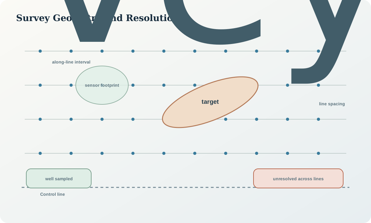
Lines usually obtain stronger spatial continuity along flight or traverse direction than across lines. A feature parallel to widely spaced lines may be poorly constrained even when profiles are individually excellent. Tie or control lines provide intersections for levelling and reveal drift or line-dependent bias. Reciprocal or repeated layouts test direction-dependent coupling and repeatability.
Survey design is conditional. An orientation phase should include pass, modify and stop rules. For example: continue only if repeated control observations fall within a declared tolerance, navigation uncertainty is small relative to the target wavelength, and the predicted model difference remains resolvable after measured field noise. “Collect first, decide later” makes geometry errors expensive and sometimes irreversible.
Spatial sampling and aliasing
Sampling replaces a continuous field with discrete observations. A sinusoidal component needs more than two samples per cycle for stable recognition in the presence of noise, irregular spacing and unknown phase. Sampling exactly at the theoretical minimum can make an alternating signal appear constant or reverse its apparent wavelength. Practical design therefore includes margin and considers the anti-alias behaviour of the instrument footprint and acquisition system.
Line spacing and along-line spacing control different directions. A dense along-line sample rate does not compensate for wide cross-line spacing. Irregular positions can reduce exact periodic aliasing but do not create sensitivity where no measurements exist. Gridding later cannot recover unobserved bandwidth; it only interpolates under a model.
Temporal sampling matters in electromagnetic gates, seismic recording, moving-platform sensors and base-field monitoring. The acquisition clock, positioning clock and source waveform must be synchronised. A time lag becomes a spatial shift when the platform moves. Record raw high-rate observations where possible and document any onboard averaging or decimation.
Footprint, detectability and resolution
Footprint is the region that materially contributes to a measurement. Detectability asks whether a response differs from uncertainty. Resolution asks whether two features or model parameters can be distinguished. Depth of investigation is a sensitivity- and noise-dependent range, not a universal hard boundary. These terms must not be substituted for one another.
Two narrow bodies may produce a single broad anomaly when their responses overlap. The anomaly can be detectable while the bodies remain unresolved. Conversely, a spatial edge may be well located from a gradient even when property magnitude is uncertain. Resolution varies across a survey with geometry, noise, coverage and constraints; a single quoted number is rarely sufficient.
Use point-spread, checkerboard or synthetic-recovery tests cautiously. A recovery test is informative only when the synthetic feature, acquisition geometry, noise model and inversion settings reflect the actual question. Testing the same smooth model favoured by the inversion can overstate resolution. Include alternative shapes, off-line locations and property contrasts.
Height, navigation, terrain and control observations
Sensor height changes amplitude and spatial bandwidth, especially for shallow sources. Terrain clearance, antenna separation, electrode positions, source–receiver offsets and borehole deviation are therefore data, not incidental notes. Use the actual observation geometry in modelling when variations are material; a nominal constant height can create false property variations.
Navigation uncertainty has direction and correlation. A constant offset shifts a feature; short-period jitter adds noise; clock mismatch creates along-track lag; an incorrect coordinate transformation can rotate, scale or displace a whole survey. Validate coordinates against independent control points and preserve both native and transformed coordinates with transformation metadata.
Terrain affects geometry and may itself generate response through density, magnetic, electrical or elevation contrast. It also constrains safety and access. A terrain correction or drape should be based on a documented elevation surface with compatible datum and resolution. Tie lines, repeat stations, reciprocal traverses and zero-response checks should be placed where they diagnose the expected failure, not merely at convenient locations.
Worked synthetic example
A synthetic target is expected to produce a shortest decision-relevant wavelength of 120 m along survey lines and 300 m across them. A proposed design uses 50 m along-line samples and 250 m line spacing. The along-line wavelength has 120/50=2.4 samples, leaving little margin for irregularity or filtering. Across lines, only 300/250=1.2 samples span the decisive wavelength, so cross-line geometry cannot represent it reliably.
A revised design uses 25 m along-line samples and 75 m line spacing, giving 4.8 and 4 samples respectively. If navigation uncertainty is 20 m across lines, the effective cross-line location error is more than a quarter of the line spacing and must still be considered. Reducing interval alone does not solve poor positioning.
Now suppose raising the sensor from 40 m to 80 m reduces the decisive model difference from 6 units to 2 units, while measured combined uncertainty is 1.2 units. The ratio falls from 5 to 1.67. The higher survey may still detect a regional anomaly but no longer reliably separate the two target hypotheses. The acceptance rule should refer to the model difference, not only total anomaly amplitude.
Geometry and resolution audit workflow
- State the smallest decision-relevant feature and competing model difference.
- Forward-model plausible depth, contrast, strike and dip bounds.
- Identify spatial, temporal and directional bandwidth that must be retained.
- Choose line direction, spacing, interval, offsets, height and tie geometry.
- Simulate sampling at actual coordinates rather than on an ideal grid.
- Add realistic navigation, timing, height and correlated noise.
- Test off-line and unfavourably oriented targets.
- Set orientation-survey pass, modify and stop criteria.
- Record actual geometry and recompute resolution after acquisition.
Practice and review
- Sketch a narrow feature parallel to survey lines and explain why dense along-line observations may not locate it across lines.
- For a 90 m wavelength, compare 45 m, 30 m and 15 m intervals and discuss margin rather than only the theoretical minimum.
- Design a control-line layout that separates line bias from short-period random noise.
- Explain how a two-second clock offset appears when a platform travels at 60 m/s.
- Write a survey acceptance criterion based on the difference between two models and total uncertainty.
Review questions: What decision-scale bandwidth is required? Which direction is weakly sampled? How does footprint differ from interval? Is a reported depth a sensitivity boundary or an interpretation? What geometry was actually acquired? Can the survey resolve the alternatives rather than merely show an anomaly?
Sources
- Resolution analysis in geophysical inverse problems, provides the foundational linear resolution framework.
- Guidelines for reporting airborne geophysical survey geometry and processing, documents acquisition, navigation, elevation, control and processing records.
- Field geophysical methods and operational quality considerations, supports geometry, safety and field-quality planning.