C4 · Publication Volume 14
Magnetic Method Foundations
susceptibility, remanence, induced field and anomaly shape
Learning goals
The learner should be able to distinguish susceptibility, induced magnetisation and remanent magnetisation; treat the measured field as a vector-dependent quantity rather than a scalar property map; predict how source geometry and magnetisation direction affect anomaly shape; check units and sign; and identify when a simple induced-field interpretation is physically inadequate.
Magnetic data are attractive because they can be acquired continuously and can reveal strong structural continuity. They are also easy to over-interpret. The same anomaly may change sign and asymmetry with latitude, source direction, remanence, sensor height and processing. Geological interpretation must begin with the magnetisation vector and acquisition geometry.
Magnetic properties and units
Magnetisation \mathbf J is magnetic moment per unit volume, expressed in amperes per metre. For a linear isotropic induced response, \mathbf J_i=\kappa\mathbf H, where \kappa is dimensionless volume susceptibility in SI and \mathbf H is the applied field intensity. Report whether susceptibility is volume or mass based, the unit system, measurement frequency and specimen orientation. A number copied without that context can be wrong by a large factor.
Susceptibility is not a fixed rock-name constant. It depends strongly on magnetic mineral abundance, grain state, alteration, weathering and fabric. Anisotropy makes response direction-dependent. Laboratory specimens can omit coarse heterogeneity or weathered zones and may not represent the survey-scale body. Use property measurements as constraints with support and uncertainty, not exact labels assigned to every model cell.
The field commonly recorded by a scalar magnetometer is total-field magnitude near the sensor, often reported in nanotesla. A magnetic anomaly is a difference after specified reference and temporal components are removed. Gradients are changes per distance and amplify short-wavelength components and position error. Do not mix absolute field, anomaly, component and derivative units.
Induced and remanent magnetisation
Induced magnetisation tends to align with the present applied field under the simple isotropic model. Remanent magnetisation persists without that field and can have a different direction acquired through thermal, chemical, depositional or other histories. The total is \mathbf J=\mathbf J_i+\mathbf J_r. When remanence is strong, assuming \mathbf J\parallel\mathbf H can place a model body incorrectly or create an implausible geometry to compensate.
Measure remanence direction and intensity on oriented material where the interpretation consequence justifies it. Sampling orientation, core rotation, demagnetisation procedure and specimen selection are part of the evidence. A few specimens rarely prove a uniform direction throughout a large body. Forward-model plausible direction ranges and inspect whether anomaly asymmetry, lows and line-to-line behaviour require remanence.
The ratio of remanent to induced intensity is useful only with compatible units and a stated inducing field. A high ratio warns that present-field transforms may be unstable. It does not by itself determine a unique remanent direction or geological age.
Main field, components and measured anomaly
The background geomagnetic field varies in direction and magnitude across the Earth and changes through time. Processing commonly uses a declared global main-field reference for the survey epoch and position. That model removes a long-wavelength estimate; it does not remove every crustal, external or temporal contribution. Record model edition, coefficients, epoch, evaluation position and whether removal occurred before or after other corrections.
A scalar total-field perturbation is approximately the projection of the anomalous vector onto the background-field direction when the perturbation is small. Consequently, the same source can produce a positive–negative pair whose position depends on magnetisation and field direction. A map high is not necessarily directly over the source. Vector or gradient observations can add constraints but also introduce orientation and calibration requirements.
Separate three questions: what the instrument recorded, which reference contributions were removed, and what physical source remains plausible. A field named “corrected magnetics” is insufficient. The correction ledger must expose temporal, heading, lag, main-field, levelling and any transform stages.
Geometry and anomaly shape
A magnetic body is bounded by changes in magnetisation. Contacts, thickness, depth, dip, strike length and magnetisation direction control the response. Shallow sharp contrasts contain shorter wavelengths; deeper sources are broader. Thin sheets, cylinders and compact bodies have different directional behaviour, but several geometries can fit a single profile.
Profile shape should be interpreted in its acquisition direction and coordinate frame. An oblique line can widen or split a response. Sensor height and terrain clearance smooth shallow components. Closely spaced sources can interfere constructively or destructively. A quiet area may represent weak contrast, greater depth, cancellation, poor orientation or inadequate sampling.
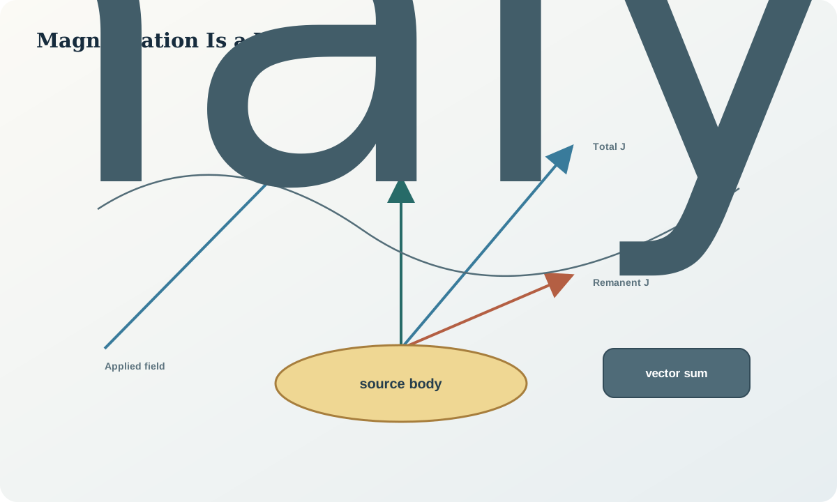
Use forward profiles before plan-map pattern matching. Compare polarity, zero crossings, extrema, gradients and line-to-line continuity. If a transform assumes induced magnetisation, also show the untransformed data and a sensitivity set with plausible remanent directions.
Worked synthetic example
A synthetic material has SI susceptibility \kappa=0.035 in an applied field intensity of 40\ \mathrm{kA/m}. The induced magnetisation magnitude under the linear isotropic assumption is
$J_i=0.035(40{,}000)=1{,}400\ \mathrm{A/m}.$
Suppose an oriented specimen suggests remanent magnetisation of 2{,}100\ \mathrm{A/m}. If it were parallel to the induced vector, total magnitude would be 3{,}500\ \mathrm{A/m}. If antiparallel, it would be 700\ \mathrm{A/m}. If perpendicular, it would be \sqrt{1{,}400^2+2{,}100^2}\approx2{,}524\ \mathrm{A/m} and point in a different direction. Adding magnitudes without vector direction could therefore be seriously misleading.
The remanent-to-induced intensity ratio is 2{,}100/1{,}400=1.5. This flags a material sensitivity test: model a range of remanent directions, include property uncertainty and compare predicted anomaly shapes. It does not justify applying the specimen direction uniformly to an unsampled body.
Magnetic-foundation audit workflow
- Identify whether each field is absolute, anomaly, component, gradient or transform.
- Confirm unit system, sign, coordinate axes, sensor orientation and height.
- Define susceptibility conditions and the spatial support of property samples.
- Separate induced and remanent magnetisation as vectors.
- Record the background-field direction, magnitude, epoch and reference model.
- Forward-model plausible source geometries and magnetisation directions.
- Compare profiles, polarity and zero crossings before map transforms.
- Test whether remanence, anisotropy or multiple sources are required.
- State which observation could discriminate direction, depth and geometry.
Practice and review
- Compute induced magnetisation for
\kappa=0.012andH=45\ \mathrm{kA/m}. - Draw vector sums for parallel, antiparallel and perpendicular remanence.
- Explain four reasons why an anomaly maximum may not lie above its source.
- List metadata required to compare two susceptibility datasets.
- Design a forward sensitivity test for a dipping body with uncertain remanence.
Review questions: Is the measured quantity a vector component or scalar magnitude? Which unit system is used? Can induced magnetisation explain the shape? How representative are property specimens? Which geometry and direction combinations remain equivalent?
Sources
- Current global main-field reference and coefficient history, documents epoch-dependent background-field modelling.
- Magnetic-property measurement definition and instrument context, supports susceptibility units and measurement metadata.
- Remanent magnetisation as a material contribution to aeromagnetic anomalies, provides a primary case demonstrating that induced-only assumptions can fail.