C4 · Publication Volume 14
Magnetic Data Processing
diurnal correction, IGRF removal, levelling, gridding, RTP and derivatives
Learning goals
The learner should be able to audit a raw-to-release magnetic processing chain; distinguish temporal, reference-field, platform and line corrections; evaluate lag, levelling and gridding from line data; explain assumptions behind common transformations; and preserve enough intermediate products to diagnose an artefact without repeating acquisition.
Processing should remove or model known non-geological contributions while preserving the signal and uncertainty needed for the decision. Every correction can also remove real geology or introduce structure when its assumptions are wrong. The safest interpretation keeps raw observations, corrected line data, crossover statistics and transform parameters together.
Raw measurements, time and navigation
A minimally useful moving-platform record includes raw field, sensor time, navigation time, position, sensor elevation, platform orientation where relevant, line and fiducial identifiers, acquisition status and quality flags. Base-field records need their own position, time base, instrument state and gap log. Synchronisation is tested, not assumed.
Lag is the displacement between recorded field and assigned position caused by sensor separation, clock offset, filtering or system latency. At platform speed v and time offset \Delta t, along-track displacement is v\Delta t. Estimating lag from geological features can confuse true asymmetry with timing error, so use reciprocal lines, calibration manoeuvres or multiple clear features and report uncertainty.
Inspect raw profiles before any smoothing. Spikes, dropouts, quantisation, manoeuvre noise, abrupt height changes and navigation jumps are easier to locate in acquisition order than in a grid. Rejected samples remain in the archive with a reason code; they are not silently deleted.
Temporal and reference-field corrections
External field variation can be estimated with a nearby base sensor or another justified reference. Suitability depends on separation, correlation, sampling rate, clock alignment and whether the variation is spatially coherent. Interpolation across a base gap is a model and needs a maximum accepted gap and uncertainty. Subtracting a noisy base series can add noise.
The global main-field reference accounts for broad position and epoch variation. Declare the model, epoch and evaluation geometry. Base correction and main-field removal address different contributions and are not interchangeable. Apply them in a documented order and preserve both the evaluated reference and corrected series.
Compare repeat and control lines before and after correction. A successful correction reduces variance attributable to the intended source without erasing repeatable geology. If a control feature changes shape, investigate clocks, spatial mismatch and filtering rather than tuning until maps look smooth.
Heading, lag, levelling and micro-levelling
Heading effects arise when the measured value depends on platform direction, sensor orientation or platform field. Estimate them from opposing directions under comparable conditions. A single additive offset may be inadequate if manoeuvres, load, current or orientation vary. Document calibration geometry and whether a heading correction is constant, line-specific or time-dependent.
Levelling reconciles systematic differences at line intersections or repeated control observations. Crossover residuals must be examined by line, direction, time and location. A least-squares adjustment can distribute discrepancies, but it cannot decide whether the cause is temporal, positional, altitude-related or geological. Large corrections are warnings, not evidence of successful cleaning.
Micro-levelling suppresses subtle line-parallel residuals after primary levelling. Because real geology can also be line-parallel, show its correction grid and spectral settings. Never release only the final smooth grid. Retain pre- and post-levelled line data, crossover tables, per-line adjustments and masks.
Gridding, derivatives and field transformations
Gridding estimates values between lines. Cell size should represent sampling density and intended bandwidth, not create apparent detail. Record coordinate reference, grid origin, extent, interpolation kernel, search radius, anisotropy, trend handling, blanking rule and any pre-filter. Inspect observed-minus-grid residuals at data locations and show areas beyond supported interpolation.
Derivatives emphasise high spatial frequencies and therefore amplify shallow signal, line noise, navigation error and gridding artefacts. Upward continuation suppresses short wavelengths and can aid scale separation; downward continuation amplifies them and can become unstable. State continuation distance, boundary treatment and stabilisation. Treat an edge-enhanced maximum as a processing response, not automatically a contact.
Transforming an anomaly to the response expected under a different field direction can simplify geometry only when magnetisation direction and other assumptions are adequate. Low inclinations, remanence, anisotropy, noise and finite boundaries can destabilise the result. Always compare the transformed product with original profiles and sensitivity alternatives.
Worked synthetic example
A synthetic aircraft travels at 70\ \mathrm{m/s}. Cross-correlation of reciprocal calibration lines indicates that the field series lags navigation by 0.8\ \mathrm s. The implied along-track shift is
$70(0.8)=56\ \mathrm m.$
If the target's shortest relevant wavelength is 140 m, the uncorrected shift is 40% of that wavelength and can materially displace gradients. Suppose uncertainty in lag is 0.15\ \mathrm s; positional uncertainty contributed by lag is then 10.5\ \mathrm m, which belongs in the spatial error budget.
After temporal and lag corrections, four line intersections have residuals 3,-2,4,-1 nT. Their mean is 1 nT and root-mean-square residual is \sqrt{(9+4+16+1)/4}\approx2.74 nT. Reporting only the mean would conceal scatter. If the decisive model difference is 2 nT at crossover-scale wavelengths, the survey does not yet support that discrimination even though the mean bias is small.
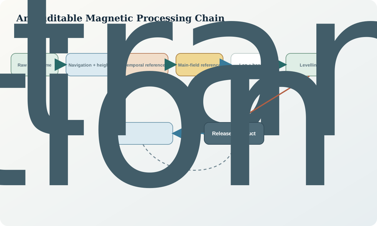
Magnetic-processing audit workflow
- Freeze raw field, time, navigation, elevation and status records.
- Test clock synchronisation and estimate lag with independent geometry.
- Flag spikes, manoeuvres, gaps and navigation failures without deletion.
- Evaluate temporal reference suitability and preserve its interpolations.
- compute the declared main-field reference for actual position and epoch.
- diagnose heading and platform effects from calibration observations.
- inspect crossover residuals before and after levelling.
- grid with documented support and examine data-space residuals.
- release correction grids, line data and assumptions beside transforms.
Practice and review
- Calculate the spatial shift for a 1.3 s offset at 55 m/s.
- Explain why subtracting a distant base series can make corrected data worse.
- Design a crossover plot that separates direction and acquisition time.
- List evidence needed before applying a present-field-direction transform.
- Describe how a line-parallel geological feature could be damaged by micro-levelling.
Review questions: Can every released value be traced to raw time and position? Which correction targets which physical contribution? Are line adjustments small relative to decisive signals? What unsupported detail did gridding create? Does a transform rely on an untested magnetisation assumption?
Sources
- Airborne geophysical survey reporting and data-submission guidance, documents raw fields, base data, lines, elevation, corrections and products.
- Current global main-field reference service, provides epoch-dependent field coefficients used in declared reference removal.
- Geomagnetism measurement and processing questions, clarifies field components, units and temporal behaviour.