C4 · Publication Volume 14
Gravity Methods
density contrast, regional and residual fields, and terrain correction
Learning goals
The learner should be able to connect density contrast and source geometry to gravity response; audit time, drift, elevation, latitude and terrain-related corrections; separate observation, regional trend and residual interpretation; assess station and elevation uncertainty; and demonstrate density–geometry non-uniqueness with a simple forward calculation.
Gravity observations respond to all mass contrast. They can constrain broad basin geometry, dense or low-density bodies and structural changes, but they do not identify composition uniquely. Small amplitudes and broad kernels make elevation, reference control and regional context central to interpretation.
Density contrast and gravitational response
For a body with density \rho_b in host density \rho_h, use \Delta\rho=\rho_b-\rho_h. Positive contrast tends to increase downward gravitational attraction; negative contrast tends to decrease it relative to the reference model. Response integrates over volume and decays with distance. Property contrast, thickness and depth trade off.
Bulk density depends on minerals, porosity, pore fluid, weathering, fractures and scale. A dry laboratory specimen may not represent an in situ saturated volume. Record measurement method, moisture condition, orientation where relevant, specimen support and uncertainty. Where property data are sparse, invert or forward-model bounded ranges rather than one exact value.
Gravity is commonly expressed as acceleration, with survey anomalies often in a smaller conventional unit. Preserve the original unit and conversion. Gradients add directional sensitivity but require precise geometry and introduce their own tensor, orientation and unit conventions.
Reference, time and drift corrections
Relative instruments measure differences and may drift with time. A base loop revisits a stable reference so drift can be estimated. The loop duration, observation sequence, reading repetitions, settling, reference value and closure residual are essential. Linear drift is only one model; abrupt steps or temperature-dependent changes require diagnosis rather than automatic interpolation.
Tidal and broader time-varying contributions can be computed or observed with declared conventions. Latitude and reference-field terms account for systematic background variation. Each correction needs a sign convention and order. A final anomaly value without the individual correction fields cannot be audited.
Network adjustment distributes loop and tie discrepancies under stated weights. Examine residuals by instrument, operator role, day, loop and location. A low overall residual can conceal a biased subgroup if weights are inappropriate. Preserve absolute reference lineage separately from relative differences.
Elevation, slab and terrain effects
Gravity changes with observation elevation and with mass between the station and a reference surface. Elevation correction uses the measured height and a declared vertical datum. A slab approximation uses an assumed reduction density; terrain correction accounts for departures of real topography from that simple reference. These operations create a conventional anomaly suited to a stated interpretation, not a direct removal of “topography” in every geological sense.
Elevation error can dominate fine gravity work. Coordinate and vertical datum, antenna or instrument offset, benchmark method and terrain-model resolution must be recorded. A terrain model that is coarse relative to nearby relief can leave structured residuals. Buildings, excavations and moving mass can also matter locally.
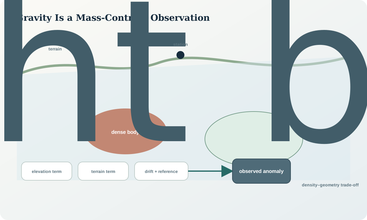
Test reduction density rather than choosing it to make geology look simple. Plot anomaly against elevation and terrain metrics, inspect repeat stations and compare results across plausible density values. A remaining correlation can reflect an inadequate correction, real geology correlated with topography or both.
Regional fields, residuals and gradients
A regional field is a model of contributions outside the target scale; a residual is the observation minus that model. There is no uniquely correct separation. Polynomial surfaces, continuation, wavelength filters and geological forward models embody different assumptions and boundary behaviour. Show the regional model, residual and sensitivity to alternatives.
Do not interpret every residual extremum as a discrete body. Edges of the survey, sparse control, terrain-correlated errors and broad unmodelled sources can create apparent targets. Cross-sections and forward models should reproduce the original observations, not only a processed residual. Independent density, structural and depth evidence can constrain the separation.
Horizontal or vertical gradients emphasise shorter wavelengths and can aid boundary localisation, but differentiation amplifies noise. Report filter, spacing, units and edge masks. A gradient maximum is a property-change indicator under assumptions; it is not a unique geological contact.
Worked synthetic example
For a scale calculation, approximate a laterally extensive horizontal layer by
$\Delta g=2\pi G\Delta\rho\,t,$
where G=6.674\times10^{-11}\ \mathrm{m^3\,kg^{-1}\,s^{-2}}, density contrast is \Delta\rho and thickness is t. A synthetic layer with \Delta\rho=250\ \mathrm{kg/m^3} and t=80\ \mathrm m gives
$\Delta g\approx2\pi(6.674\times10^{-11})(250)(80)=8.39\times10^{-6}\ \mathrm{m/s^2}.$
The same response results from \Delta\rho=125\ \mathrm{kg/m^3} and t=160\ \mathrm m under this approximation. Gravity alone cannot separate those combinations. Finite lateral extent and depth to top would change the shape, but they introduce further trade-offs.
Suppose total uncertainty at the relevant scale is 1.2\times10^{-6}\ \mathrm{m/s^2} and two structural models differ by only 0.7\times10^{-6}\ \mathrm{m/s^2}. Both can be detectable relative to background yet indistinguishable from each other. A density measurement, closer station geometry or an independent depth-sensitive method may be more valuable than additional smoothing.
Gravity audit workflow
- Verify acceleration units, sign, reference datum and coordinate frame.
- Reconcile station times, repetitions, instruments, loops and base values.
- inspect closure and drift residuals before spatial interpretation.
- preserve every temporal, latitude, elevation, slab and terrain term.
- validate horizontal and vertical positions against independent control.
- test reduction density and terrain-model resolution.
- compare several regional–residual separations at data locations.
- forward-model bounded density and geometry alternatives.
- specify independent evidence that can break density–volume trade-offs.
Practice and review
- Recalculate the layer example for
150\ \mathrm{kg/m^3}and 120 m. - Explain why a perfect base-loop closure does not prove correct elevations.
- List three causes of an anomaly–elevation correlation after correction.
- Compare a smooth regional surface with a geology-based regional model.
- Design a second observation to distinguish a thin dense layer from a thick weakly dense layer.
Review questions: Which mass contrasts contribute? How were drift and references controlled? Is the vertical datum explicit? How sensitive is the residual to reduction choices? Which density–geometry models fit within uncertainty?
Sources
- Tools and techniques for the gravitational method, provides a primary technical overview of gravity acquisition and interpretation.
- Gravity method fact sheet, explains density contrast and gravity-field applications.
- Geophysical acquisition, processing and gravity reference stewardship, documents quality benchmarks, calibration and reference networks.