C4 · Publication Volume 14
Electrical Resistivity and Induced Polarisation
conductivity, chargeability, arrays and depth of investigation
Learning goals
The learner should be able to relate current injection and potential measurement to apparent resistivity; explain sensitivity and depth behaviour of electrode arrays; distinguish conductivity from chargeability; diagnose contact, coupling and cultural noise; and interpret two-dimensional or three-dimensional models as regularised explanations rather than direct images.
Electrical methods are sensitive to connected pore fluids, conductive minerals, clay, porosity, saturation and geometry. Induced polarisation adds sensitivity to delayed electrochemical or interfacial response. Neither response uniquely identifies a commodity or lithology.
Current, potential and apparent resistivity
A controlled current I is injected through source electrodes and a potential difference \Delta V is observed between receiver electrodes. For a declared array over a homogeneous reference medium, apparent resistivity is
$\rho_a=K\frac{\Delta V}{I},$
where K is a geometric factor in metres. Apparent resistivity is a data transform. In heterogeneous ground it is not the true resistivity at a point or a simple average under the array.
Conductivity is the reciprocal of resistivity only for compatible scalar, linear conditions. Clay surface conduction, metallic pathways, pore-fluid salinity, saturation, anisotropy and frequency dependence can complicate effective response. Temperature and electrode polarisation may matter. Record current waveform, amplitude, polarity, cycle, receiver window, electrode coordinates, contact resistance and units.
Sign reversals and very small potentials require careful handling. The current and voltage channels should retain polarity. Stacking reduces some random noise but does not remove coherent coupling or an incorrect geometric factor. Reciprocal measurements provide a valuable data-space check when geometry permits.
Arrays, sensitivity and depth of investigation
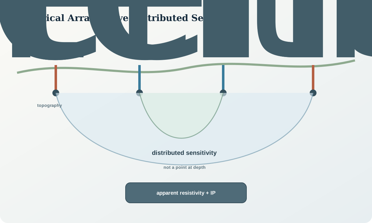
An electrode configuration defines a sensitivity pattern with positive and negative regions. Array length, spacing and orientation influence investigation depth, lateral resolution and signal level. A datum plotted at a conventional pseudodepth is not a local measurement at that point. Inversion is needed to relate the full sensitivity to a property model.
Topography and exact electrode coordinates can materially alter response. Use measured positions and elevation rather than idealised regular spacing when differences matter. Two-dimensional inversion assumes negligible variation perpendicular to the line; a conductor oblique to the line can violate that assumption. Cross-lines or three-dimensional acquisition can test it.
Depth of investigation varies with current strength, noise, geometry, conductivity structure and inversion constraints. Report a sensitivity or perturbation test, not only the bottom of a coloured section. Cells below useful sensitivity should be masked or visibly de-emphasised.
Induced polarisation and chargeability
After an applied current changes, voltage can decay over time because charge has accumulated at interfaces or within electrochemical systems. Time-domain chargeability is commonly derived by integrating or averaging secondary voltage over declared gates and normalising by a primary voltage. Frequency-domain measurements examine amplitude and phase variation with frequency. The exact reported quantity depends on waveform, gates and convention.
Chargeability can arise from disseminated electronically conductive grains, clay, membrane effects and other interfaces. It does not uniquely indicate sulphide mineralisation. Resistivity and chargeability should be interpreted together because current flow and signal-to-noise affect the measured IP response. A chargeable region may be poorly excited if surrounded by very resistive material.
Record full decay or spectral data where possible. A single scalar chargeability can hide early-time coupling, late-time noise or mixed mechanisms. Inspect gate uncertainty, sign, repeatability and residual waveform after removing the transmitter response.
Contact, coupling, noise and field controls
High or unstable contact resistance limits current and can introduce voltage noise. Record contact tests before and during acquisition. Electrode movement, drying ground, cable leakage and poor isolation can cause drift. Current and potential cables can couple capacitively or inductively, especially at early times or higher frequencies.
Infrastructure, grounded fences, pipes and power systems can redirect current or add coherent noise. Their effects depend on geometry, so map them and inspect reciprocal or reversed arrays. Simply rejecting high values may remove real geological response while retaining less obvious cultural distortion.
Field controls include current waveform diagnostics, injected current stability, repeat and reciprocal observations, contact resistance, receiver saturation, standard loops or test circuits where appropriate, and remote-reference or synchronised monitoring for natural-field noise. Acceptance rules should distinguish acquisition failure from genuine nonlinear or heterogeneous response.
Worked synthetic example
A synthetic four-electrode datum has geometric factor K=12\ \mathrm m, measured potential \Delta V=0.075\ \mathrm V and injected current I=0.050\ \mathrm A. Its apparent resistivity is
$\rho_a=12\frac{0.075}{0.050}=18\ \Omega\mathrm m.$
If the voltage uncertainty is 0.004\ \mathrm V and current uncertainty is negligible for this example, relative measurement uncertainty is about 0.004/0.075=5.33\%, giving roughly 0.96\ \Omega\mathrm m before geometry and positioning uncertainty.
For a separate synthetic IP datum, average secondary voltage in the declared gate is 0.028\ \mathrm V and primary voltage is 0.700\ \mathrm V. Normalised chargeability is 0.028/0.700=0.040\ \mathrm{V/V}, or 40 mV/V. Changing the gate could change the value, so the scalar is incomplete without waveform and gate definition.
Electrical and IP audit workflow
- Reconcile electrode identities, coordinates, elevations and array geometry.
- verify current polarity, waveform, timing, voltage unit and geometric factor.
- inspect contact resistance, saturation, leakage and current stability.
- compare repeats, reciprocals and reversed configurations.
- retain apparent data, full decays or spectra and uncertainty.
- include actual topography and three-dimensional context where required.
- define inversion error floors, bounds and regularisation before viewing geology.
- mask low-sensitivity regions and inspect data-space residuals.
- compare fluid, clay, mineral and cultural explanations.
Practice and review
- Calculate
\rho_aforK=25m,\Delta V=0.032V andI=0.080A. - Explain why pseudodepth is not a measurement depth.
- List four mechanisms that can produce a chargeable response.
- Design field tests for a conductor coincident with a grounded fence.
- State how a two-dimensional assumption could fail for an oblique body.
Review questions: What array and waveform produced the datum? Are coordinates exact? Which volume has sensitivity? Is chargeability supported by the decay shape? What non-geological conductors remain viable? Which cells are constrained by data rather than regularisation?
Sources
- Parallel modelling for electrical resistivity and induced-polarisation characterisation, provides a primary example of sensitivity and joint interpretation.
- Surface geophysical method overview, relates electrical response to subsurface properties and applications.
- Field geophysical activities and quality considerations, supports controlled acquisition and field records.