C4 · Publication Volume 14
Electromagnetics
time and frequency domains, conductors, coupling and decay
Learning goals
The learner should be able to explain induction, diffusion and secondary fields; distinguish time-domain and frequency-domain observations; evaluate transmitter–receiver coupling and system geometry; relate conductivity, permeability and thickness to response; and audit conductivity-depth products without equating an inversion section with geology.
Electromagnetic surveys can detect conductive pathways and map cover architecture over a wide range of scales. Their response depends on waveform, frequency or time gate, source moment, orientation, motion, conductive geometry and background. A strong conductor can be invisible if poorly coupled, while a weak broad conductor can dominate late-time response.
Induction, diffusion and secondary fields
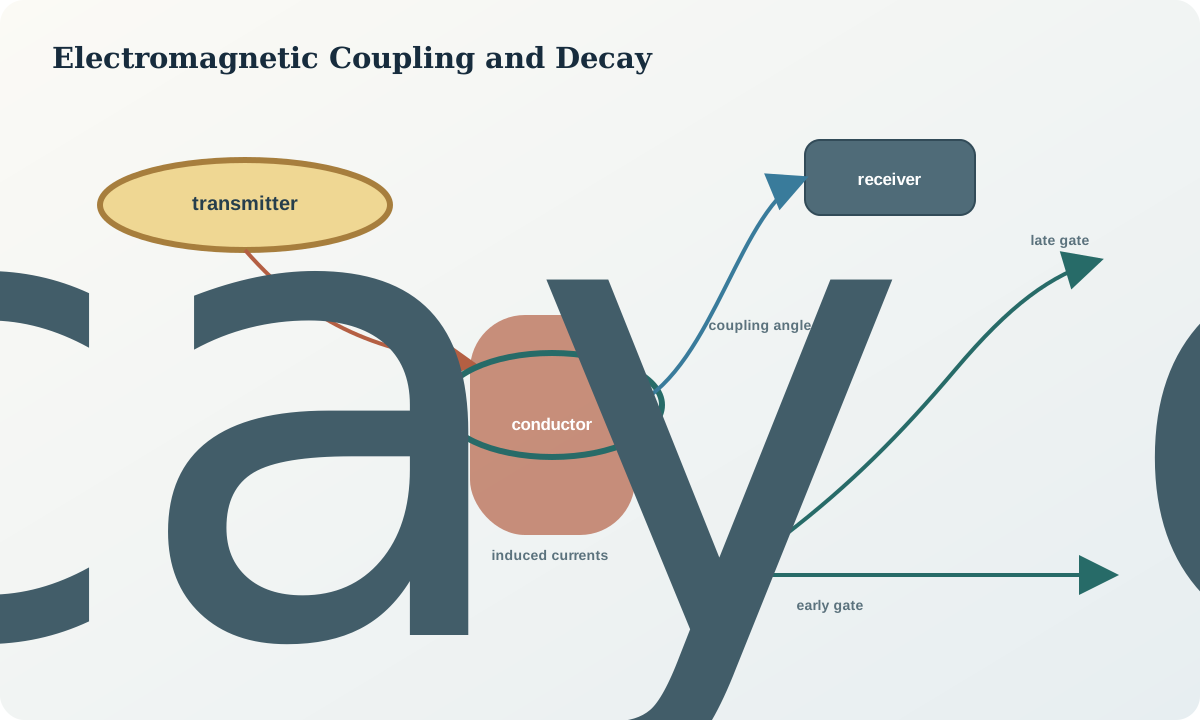
A changing transmitter current creates a primary magnetic field. Conductive ground supports induced currents that produce a secondary field measured by a receiver. The induced currents diffuse outward and decay through time; their distribution depends on conductivity, magnetic permeability and geometry. The receiver records a component or rate of change determined by orientation and system response.
Primary-field removal is often a major challenge because the secondary response may be small. Transmitter waveform, receiver transfer function, timing and geometry must be known. Conductivity is not the only control: a thin high-conductivity sheet and a thicker moderate conductor can have similar conductance and response over limited bandwidth.
Near-surface conductors can shield or distort deeper response. Magnetic permeability and induced polarisation can affect some systems. A one-dimensional layered assumption may be useful for broad subhorizontal cover but can fail near steep conductors, faults or strong lateral variation.
Time-domain and frequency-domain observations
Time-domain systems transmit a pulse or switched waveform and observe secondary decay in gates after or during current change. Early gates emphasise rapid and shallow or weak responses but are vulnerable to system transients; later gates can contain information on stronger or deeper conductors but have lower signal and more ambient noise. Gate centre alone is insufficient; record gate width and stacking.
Frequency-domain systems transmit one or more sinusoidal frequencies and measure in-phase and quadrature components, amplitude and phase, or related ratios. Lower frequencies generally permit broader diffusion in a conductive medium, while higher frequencies emphasise shallower response. Frequency coverage and noise determine whether conductivity and geometry can be separated.
Time and frequency representations are mathematically related for a linear system with adequate bandwidth, but practical surveys sample limited, noisy ranges with different waveforms and calibration. Do not combine them without matching conventions, units, sign, orientation and system response.
Coupling, geometry and system calibration
Inductive coupling depends on the angle and distance among transmitter, receiver and conductor. A plate aligned unfavourably to the primary field may carry little induced current. Flight-line direction, loop orientation and source–receiver separation therefore affect detectability. Acquire orthogonal or multiple-component observations where directional ambiguity matters.
Platform motion, pitch, roll, yaw, terrain clearance and transmitter–receiver geometry modulate response. Nearby metal and power systems can create coherent signals. Calibration includes waveform and moment, timing, receiver gain and phase, orientation, primary-field compensation and system drift. A calibration coefficient is valid only for the configured system.
Inspect raw waveforms or channel profiles, system monitors, altitude and orientation together. A response locked to manoeuvres or power infrastructure is not made geological by a smooth conductivity image. Repeated calibration lines and high-altitude or zero-response checks help separate system from ground.
Conductivity–depth interpretation and uncertainty
A uniform half-space illustrates diffusion scale. For a non-magnetic medium, a common characteristic depth is approximately
$\delta\approx503\sqrt{\frac{\rho}{f}}\ \mathrm m,$
with resistivity \rho in ohm metres and frequency f in hertz. This is a scale, not the survey's unique depth of investigation. Actual sensitivity depends on source–receiver geometry, layered conductivity, bandwidth and noise.
Conductivity-depth images and layered inversions distribute response with depth using constraints. Smoothness, fixed layer boundaries, bounds and starting models can dominate where data sensitivity is weak. Show observed and predicted channels, normalised residuals, sensitivity or depth-of-investigation metrics, and alternative regularisation.
Interpret conductive and resistive features through hypotheses. Saline fluid, clay, graphite, interconnected sulphides, weathering and infrastructure may overlap in response. Use geology, borehole conductivity, IP, magnetics, geochemistry or seismic information to discriminate rather than assigning a material from conductivity alone.
Worked synthetic example
For a synthetic uniform medium with \rho=100\ \Omega\mathrm m observed at f=1{,}000 Hz, the characteristic depth is
$\delta\approx503\sqrt{100/1{,}000}=159\ \mathrm m.$
At 4,000 Hz it is about 79.5 m. Doubling the frequency does not halve the scale; the dependence is inverse square root. These numbers do not guarantee detection at those depths.
Now consider two thin-sheet models with conductance S=\sigma t. Model A has \sigma=1\ \mathrm{S/m} and thickness 8 m, so S=8 S. Model B has \sigma=0.25\ \mathrm{S/m} and thickness 32 m, also 8 S. Over limited bandwidth their responses may be similar. Additional late-time data, geometry or a borehole constraint is needed before thickness and conductivity can be claimed separately.
Electromagnetic audit workflow
- Identify recorded component, unit, sign, waveform, gates or frequencies.
- reconcile transmitter–receiver positions, orientation, moment and clocks.
- inspect system transients, primary-field compensation and calibration.
- map altitude, attitude, infrastructure and line-direction dependence.
- compare repeated and orthogonal observations where available.
- retain raw channels and predicted data beside conductivity images.
- test layered, plate and lateral-variation alternatives.
- map sensitivity and depth limits rather than the model mesh boundary.
- seek independent evidence for conductor material and geometry.
Practice and review
- Calculate the characteristic depth for 25
\Omegam at 400 Hz. - Explain why a steep conductor can be missed by an unfavourably oriented loop.
- List five system or cultural effects that can imitate ground response.
- Compare two conductivity–thickness combinations with equal conductance.
- Design an independent test to distinguish saline water from graphite.
Review questions: What field component and gate were measured? Is system geometry known? Can primary-field leakage explain the feature? Which conductivity–geometry models fit? Where does regularisation dominate? What evidence identifies the conductor rather than only its response?
Sources
- Official airborne electromagnetics acquisition, processing and inversion guidance, documents system calibration, processing, noise fitting and model uncertainty.
- Airborne electromagnetic survey data and product structure, illustrates raw channels, geometry, conductivity products and depth metrics.
- Electromagnetic methods review, provides a primary synthesis of time- and frequency-domain applications and limitations.