C4 · Publication Volume 14
Seismic Methods
velocity, reflection, refraction, resolution and hard-rock limitations
Learning goals
The learner should be able to relate elastic properties to wave velocity and impedance; distinguish reflection and refraction questions; design source–receiver geometry for target depth and wavelength; audit picks and processing; and explain why a coherent seismic event can have multiple geological interpretations, especially in structurally complex hard rock.
Seismic observations contain travel time, amplitude, phase, frequency, polarisation and attenuation information. They are not photographs. Acquisition and processing construct an image under velocity, geometry and wave-propagation assumptions that must remain attached to the interpretation.
Wave propagation, velocity and impedance
Compressional and shear waves respond differently to elastic moduli and density. Velocity can vary with mineralogy, porosity, fractures, fluids, pressure, weathering and direction. Anisotropy makes travel time depend on propagation direction. Attenuation reduces high frequencies and can change phase.
Acoustic impedance is Z=\rho v for the relevant wave mode under a simple normal-incidence approximation. A boundary produces reflected energy when impedance changes; a large velocity contrast without suitable geometry or bandwidth does not guarantee a clear mapped reflector. Gradual transitions may have weak reflections even when total property change is large.
Wavelength is \lambda=v/f. Higher frequency offers shorter wavelength and potentially finer resolution, but attenuation usually increases and source energy may fall. State the frequency band actually present at target depth rather than the nominal source band.
Reflection and refraction
Reflection analysis uses energy returning from impedance contrasts. Two-way time must be converted to depth with a velocity model. Dip, out-of-plane structure and anisotropy can misplace events. Migration or equivalent imaging moves energy according to assumed propagation; it does not guarantee correct geology if velocity is wrong.
Refraction analysis uses first arrivals that travel along or through faster regions. Conventional interpretations work best when velocity generally increases with depth and interfaces are sufficiently continuous. A hidden low-velocity layer can be poorly constrained. Tomographic inversion relaxes some geometry but remains non-unique and regularised.
Use both data types where possible. First arrivals can constrain near-surface and broad velocity structure for reflection processing; reflections can add interface detail. Surface waves and converted phases may be signal or noise depending on the question, but they should not be removed without diagnosing their contribution.
Acquisition, bandwidth and resolution
Source type, energy, repeatability and coupling determine emitted bandwidth. Receiver spacing, aperture, orientation and sampling rate determine captured wavefield. Offsets must span the angles and depths needed for the question. Fold is not a universal quality number; repeated traces help only if geometry samples useful reflection points and static variations are controlled.
Near-surface weathering causes time shifts and attenuation. Survey elevation and source and receiver coordinates require precise vertical and horizontal control. In hard rock, steep structures, scattering, low impedance contrast, strong surface waves and access constraints can limit conventional layouts. Three-dimensional geometry may be necessary to avoid out-of-plane ambiguity.
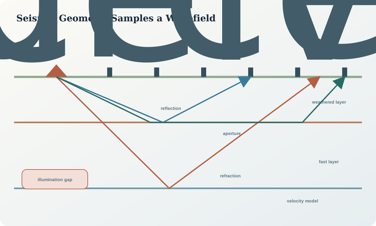
Vertical resolution is often related to a fraction of dominant wavelength, but the useful value depends on interference, signal-to-noise, processing and criterion. Horizontal resolution depends on aperture, depth, frequency and imaging. Demonstrate recovery with synthetic events that include realistic noise and alternative dips.
Processing, statics and interpretation limits
A processing sequence may include geometry assignment, amplitude recovery, deconvolution, noise attenuation, static correction, velocity analysis, normal-moveout correction, stacking and migration. The order and parameters can change continuity and apparent dip. Preserve representative raw gathers and intermediate panels so an interpreter can see what created an event.
Static corrections address near-surface time variation. Incorrect statics can break or fabricate reflectors. Aggressive coherent-noise removal can erase steep geological events; automatic gain can make noise look significant; stacking can suppress nonconforming but real arrivals. Test parameters on known synthetic and field control events.
Interpretation uses event termination, continuity, amplitude, phase, velocity and structural context, but each attribute has acquisition dependence. A blank zone may be homogeneous, steep, attenuating, poorly illuminated or damaged by processing. Map confidence and alternative event correlations rather than tracing a single preferred horizon through every gap.
Worked synthetic example
Synthetic layer 1 has density 2{,}400\ \mathrm{kg/m^3} and compressional velocity 3{,}000\ \mathrm{m/s}, giving impedance Z_1=7.2\times10^6\ \mathrm{kg\,m^{-2}\,s^{-1}}. Layer 2 has 2{,}700\ \mathrm{kg/m^3} and 5{,}000\ \mathrm{m/s}, giving Z_2=13.5\times10^6 in the same units.
At normal incidence, the simple amplitude reflection coefficient is
$R=\frac{Z_2-Z_1}{Z_2+Z_1}=\frac{6.3}{20.7}\approx0.304.$
The positive sign follows the stated polarity convention and impedance increase. Real amplitude also depends on angle, source, coupling, attenuation, processing and anisotropy.
If dominant frequency at depth is 75 Hz and velocity is 4{,}500\ \mathrm{m/s}, wavelength is 60 m. A nominal quarter-wavelength separation is 15 m, but this is not a guaranteed bed-thickness resolution. The learner must test interference, noise, bandwidth and imaging geometry before claiming two interfaces are resolved.
Seismic audit workflow
- verify source and receiver coordinates, elevations, clocks and orientation.
- inspect source signature, coupling, dead channels and raw gathers.
- map frequency content, offsets, azimuths and illumination at target depth.
- audit statics, velocity analysis and rejected traces.
- compare pre- and post-noise-removal panels for damaged signal.
- retain the velocity model and parameters used for depth conversion and imaging.
- test steep, out-of-plane, anisotropic and low-velocity alternatives.
- map event-pick uncertainty and processing-sensitive intervals.
- seek independent property or borehole constraints before assigning geology.
Practice and review
- Compute impedance and
Rfor two synthetic layers of your own design. - Calculate wavelength for 6,000 m/s at 50 and 150 Hz.
- Explain how a low-velocity hidden layer challenges simple refraction interpretation.
- List processing operations that could erase a steep event.
- Design an observation to test whether a blank zone is poor illumination or homogeneous rock.
Review questions: Which wave mode and band are present? What geometry illuminates the target? How uncertain is the velocity model? Can statics or filtering explain the event? Which alternative correlations fit? Is depth supported independently?
Sources
- Seismic reflection and refraction site characterisation, provides a primary comparison of reflection and refraction methods.
- Seismic methods for structural investigation, reviews travel-time, velocity and structural interpretation.
- Coincident seismic reflection and refraction studies, demonstrates complementary constraints and interpretation limits.