B5 · Publication Volume 10
Elements, Ionic Radius and Valence
periodic behaviour, substitution and compatibility
Learning goals
After this lesson, you should be able to explain why elements with similar charge and size may substitute for one another, why coordination changes an effective ionic radius, how crystal-site geometry and bonding constrain trace-element residence, and why compatibility is a property of a phase assemblage and conditions rather than an eternal label attached to an element.
You should also be able to calculate a mineral-melt and bulk partition coefficient, use a simple batch-melting mass balance, distinguish lattice substitution from inclusions or surface contamination, and design observations that test where an element resides. The target is not memorisation of a periodic table of “mobile” and “immobile” elements. It is a transferable model connecting electronic structure, site occupancy, phase proportions and process.
Periodic behaviour and charge
An element's atomic number fixes the number of protons. Chemical behaviour depends on electron configuration, oxidation state and bonding environment. Across a period, effective nuclear charge generally increases and atomic size tends to decrease; down a group, additional electron shells generally increase size. These trends orient reasoning but do not replace a structural model.
An oxidation state is a formal electron-accounting convention. It is not always a directly measured ionic charge. Iron may occur mainly as Fe(II) or Fe(III), sulfur may span reduced sulfide to oxidised sulfate, and uranium may change coordination and solubility with oxidation state. If valence controls the interpretation, measure or constrain it rather than treating total elemental concentration as a complete description.
Charge balance matters in a crystal. Substitution of one ion for another with the same charge can be approximately charge neutral. A heterovalent substitution requires coupled substitution, vacancies, interstitials or a change elsewhere. A formula normalised without a defensible valence assignment can produce a numerically tidy but chemically impossible site allocation.
Ionic radius, coordination and crystal sites
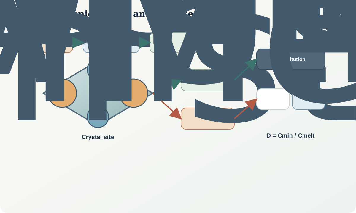
An effective ionic radius depends on oxidation state, coordination number and, for some ions, spin state. A radius tabulated for sixfold coordination cannot be transferred silently to an eightfold site. Crystal sites have geometry, bond length, charge environment and distortion limits. Substitution is favoured when an entering ion can satisfy these constraints with tolerable elastic and electrostatic cost.
The familiar size-similarity heuristic is therefore conditional. A modest radius mismatch may be accepted at high temperature because the lattice is expanded and configurational entropy matters; a similar mismatch may be rejected at lower temperature. Charge mismatch can dominate size similarity. Site occupancy may also depend on competition from abundant major elements and on whether charge compensation is locally available.
Three observations that look like “element in mineral” must be separated: true lattice substitution, microscopic inclusion of another phase, and material on a fracture or surface. Bulk dissolution alone may not distinguish them. Spatially resolved chemistry, imaging, diffraction or sequential preparation can test the host.
Partition coefficients and compatibility
For element i between a mineral and a coexisting melt,
$D_i^{min/melt}=\frac{C_i^{min}}{C_i^{melt}}.$
Under the stated conditions, D>1 means the mineral contains a higher concentration than the melt and the element is compatible in that mineral. D<1 means it is incompatible in that mineral. A bulk coefficient for an assemblage is
$\bar D_i=\sum_j \phi_jD_i^j,$
where \phi_j is the mass fraction of phase j in the relevant solid assemblage. The sum of phase fractions must be one on the same basis.
Neither coefficient is universal. It varies with mineral composition, pressure, temperature, oxygen fugacity, melt polymerisation, water content and the concentration range over which the model applies. A trace element may behave compatibly in one mineral-bearing assemblage and incompatibly after that mineral disappears. The geological question must therefore specify phases and conditions.
Linking site preference to process
Site-scale reasoning becomes useful when it predicts a process-scale pattern. Large ions with low charge may fit poorly into common compact silicate sites and remain in melt during early crystallisation. High-field-strength ions combine charge and size in ways that may favour accessory phases. Rare-earth patterns can reflect systematic radius change across a valence series, but an observed pattern can also be controlled by accessory-mineral inheritance, alteration or analytical normalisation.
A lattice-strain view treats partitioning across a related ion series as an energetic response to radius mismatch around an optimum site radius. This explains why a smooth curve can arise without assigning a separate mechanism to every element. The curve is evidence for a site model only if the relevant ions share charge and coordination and the phases were in suitable equilibrium.
Do not reverse the inference automatically. A smooth pattern does not prove a unique mineral assemblage, and a depletion does not prove that a phase fractionated. Source composition, partial melting, mixing and later alteration can create similar signals. Test the predicted mineral hosts and complementary reservoirs.
Sampling and analytical design
Begin with the object: whole rock, mineral separate, growth zone, inclusion, alteration rim or solution. A whole-rock analysis averages phases according to sampled mass. A spot analysis samples a small interaction volume that may cross zoning or an inclusion. A mineral separate can retain intergrowths and coatings. Record grain size, separation criteria, imaging and rejected material.
Select elements according to hypotheses, not merely because an instrument reports them. If coupled substitution is proposed, measure both substituting and charge-balancing constituents. If accessory-phase control is possible, include petrographic counts or imaging. If valence matters, pair total concentration with a valence-sensitive method or an independently constrained redox environment. Include blanks, duplicates and reference materials appropriate to the matrix and concentration range.
Normalisation can reveal patterns but also introduces dependence. A ratio with a small or variable denominator can exaggerate noise. Reference-composition normalisation requires a declared version and does not remove sampling or analytical uncertainty. Plot raw concentrations and uncertainties alongside derived patterns.
Worked synthetic example
A synthetic source contains three solid phases with mass fractions 0.60, 0.25 and 0.15. Their partition coefficients for element X relative to melt are 0.10, 0.40 and 2.00. The bulk coefficient is
$\bar D_X=(0.60)(0.10)+(0.25)(0.40)+(0.15)(2.00)=0.46.$
Suppose 20% equilibrium batch melting occurs and the bulk coefficient is treated as constant. For initial source concentration C_0, the melt concentration is
$\frac{C_l}{C_0}=\frac{1}{\bar D+F(1-\bar D)} =\frac{1}{0.46+0.20(0.54)}=1.7606.$
The residual solid has C_s/C_0=\bar D(C_l/C_0)=0.8099. The mass-balance check is
$F\frac{C_l}{C_0}+(1-F)\frac{C_s}{C_0} =(0.20)(1.7606)+(0.80)(0.8099)=1.0000.$
The calculation says the melt is enriched relative to the source under this model. It does not prove equilibrium, constant phase proportions, a real source composition or absence of accessory-phase exhaustion. The phase with D=2 strongly affects \bar D despite its smaller abundance. A defensible application would test whether that phase is present throughout melting and whether element X truly resides in it.
Interpretation workflow
- Define the sampled object, preparation and analytical basis.
- State the proposed host site or phase and its charge, coordination and compositional range.
- Check charge balance and possible coupled substitutions.
- Separate lattice residence from inclusions, intergrowths and surface material.
- State the pressure, temperature, phase and melt or fluid composition associated with any partition coefficient.
- Calculate the bulk coefficient from phase mass fractions on a common basis.
- Close the mass balance and display sensitivity to phase proportion and
D. - Seek complementary evidence in residue, product, zoning or another reservoir.
- Report alternatives such as inheritance, mixing or alteration.
The final interpretation should name the level of confidence. “Compatible” is incomplete; write “compatible in the modelled assemblage over the stated conditions” and preserve the evidence supporting those conditions.
Failure modes and uncertainty
Common failures include using a radius without its coordination and valence, treating oxidation state as total element concentration, applying a partition coefficient outside its calibrated range, averaging phase proportions that do not coexist, and assuming a smooth normalised pattern has a unique cause. Another failure is selecting a least-altered sample after seeing the desired pattern, which makes the test circular.
Uncertainty enters through sampling heterogeneity, phase abundance, zoning, analytical calibration, detection limits and model parameters. Sensitivity may be nonlinear when a high-D accessory phase appears or disappears. Report scenarios with and without that phase rather than hiding the discontinuity inside a single standard deviation.
A precise spot result can be unrepresentative of the rock, while a representative whole-rock result can obscure the controlling microdomain. The appropriate support depends on the geological question. Use nested observations when possible: field relation, petrography, phase chemistry and bulk balance.
Practice and review
- For three ions of equal charge but different effective radius, sketch a qualitative lattice-strain curve and identify the assumptions required to interpret it.
- Design a coupled-substitution test in which a divalent ion replaces a trivalent ion. Which additional site or vacancy measurement is needed?
- Recalculate the synthetic example if the 15% high-
Dphase is absent and the other phases are renormalised. Explain the geological consequence. - A mineral separate has a high concentration of an element but imaging shows sparse inclusions. Propose measurements that distinguish lattice residence from inclusion control.
- Write a two-column evidence ledger for the claim “element Y was incompatible during melting”: support on the left, possible contradiction on the right.
For the completion exercise, create a synthetic four-phase source with declared phase proportions and coefficient ranges. Propagate low, central and high cases through a batch-melting calculation, verify mass closure, and write one paragraph that separates the numerical result from its geological interpretation.
Sources and further reading
- Shannon, Revised effective ionic radii, coordinated radius framework used in crystal-chemical reasoning.
- Ringwood, Principles governing trace-element distribution during magmatic crystallisation90036-3), early systematic treatment of charge, size and complex formation.
- Blundy and Wood, Prediction of crystal-melt partition coefficients, lattice-strain formulation for mineral-melt partitioning.
- Wood and Blundy, Effect of cation charge on crystal-melt partitioning00294-1), charge-dependent extension of site-partition reasoning.
- Blundy and Wood, Partitioning of trace elements between crystals and melts00129-8), review linking crystal chemistry to igneous processes.