B5 · Publication Volume 10
Partitioning, Fractionation and Mass Balance
partition coefficients, fractionation and mass-balance reasoning
Learning goals
After this lesson, you should be able to distinguish partitioning from fractionation, select an equilibrium, batch, fractional or mixing model, calculate a bulk distribution coefficient, close a mass balance, and explain why concentration change is not automatically mass gain or loss. You should also be able to recognise compositional closure and denominator effects.
The central habit is to define system boundaries before choosing an equation. A reservoir may exchange heat but not mass, exchange selected dissolved components, lose crystals, gain fluid, or mix with another material. Each boundary produces a different model. An equation that fits a trend is not evidence that its boundary conditions occurred.
Reservoirs, fluxes and system boundaries
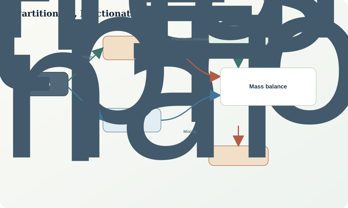
A reservoir is a declared quantity of material with composition and mass. A flux transfers material across the boundary. Partitioning distributes a component between coexisting phases. Fractionation changes one reservoir relative to another because phases or reaction products are separated. Mixing combines reservoirs. Reaction can redistribute components without changing total system mass, while open-system addition or removal changes inventory.
Draw the system before calculating. Identify source, product, residue and any external input or output. State whether masses are initial, instantaneous or final. A concentration has dimensions of component mass divided by sample mass; it cannot reveal inventory without the denominator mass. Ten grams per tonne in a shrinking rock mass may represent loss, constancy or gain of the component.
The conservation statement for component i is
$M_0C_{i,0}+\sum M_{in}C_{i,in}=\sum M_{out}C_{i,out}+M_fC_{i,f},$
using consistent units and basis. Every simplified equation is a special case of this ledger.
Equilibrium and fractional models
For equilibrium batch melting with melt fraction F and constant bulk coefficient \bar D,
$C_l=\frac{C_0}{\bar D+F(1-\bar D)}.$
The melt remains in equilibrium with the residue until separation. Fractional melting instead removes infinitesimal melt increments, producing a different aggregate. For Rayleigh fractional crystallisation with a remaining melt fraction F and constant bulk coefficient,
$C_l=C_0F^{\bar D-1}.$
This form assumes instantaneous crystals are removed from further equilibration. If crystals remain, if \bar D changes as phases change, or if recharge and assimilation occur, the simple curve is inadequate.
Equilibrium and fractional are end-member models. Natural systems may show imperfect separation, trapped melt, boundary-layer effects or repeated recharge. Use the simplest model that can be contradicted by the available data, then add complexity only when residual patterns require it.
Mixing and compositional closure
For binary mixing of two materials on the same mass basis,
$C_{mix}=fC_A+(1-f)C_B,$
where 0\le f\le1. Concentrations mix linearly only when the component and total-mass basis are compatible. Ratios generally follow curved relations because both numerator and denominator change. An apparent straight line in ratio-ratio space may therefore reflect the chosen denominators rather than a unique process.
Major-element analyses are commonly closed to a constant total such as 100%. Increasing one component forces the relative proportions of others downward even if their absolute inventory is unchanged. Standard correlations and distances applied directly to closed proportions can be misleading. Log-ratio reasoning compares relative information while avoiding assignment of a privileged total, but zeros, detection limits and mixed analytical bases still require explicit treatment.
Never renormalise away a low analytical total before investigating volatiles, alteration, incomplete digestion or reporting basis. Preserve both the measured total and any normalised table.
Alteration and immobile-reference mass balance
When a rock gains or loses total mass, raw before-after concentrations do not measure component transfer. An immobile-reference method estimates the mass change from one or more components assumed not to have moved. If reference component r is conserved,
$\frac{M_f}{M_0}=\frac{C_{r,0}}{C_{r,f}}.$
The final inventory of component i relative to its initial inventory is
$\frac{M_fC_{i,f}}{M_0C_{i,0}}= \frac{C_{r,0}}{C_{r,f}}\frac{C_{i,f}}{C_{i,0}}.$
A gain-loss value may be written as this ratio minus one. The reference is a geological hypothesis, not a magic element. Mechanical sorting, resistant accessory minerals, detrital input and intense reaction can move commonly assumed immobile components. Test several references, mineral hosts and spatial trends.
An isocon graph compares altered and precursor concentrations. A line through components judged immobile estimates the relative mass factor. The chosen precursor must be genuinely comparable; selecting it solely because it makes the diagram tidy is circular.
Data design and quality checks
Record wet, dry, volatile-free and oxide-converted bases separately. Confirm whether iron is reported as FeO, Fe2O3, total iron in one convention or measured valence species. For partial digestion, do not compare results with total digestion as if they represented the same inventory. Detection-limit substitutions can distort ratios and log transforms.
Before modelling, check analytical totals, blanks, duplicates, reference materials and between-batch drift. Plot individual samples and petrographic classes. Identify cumulates, xenoliths, veins, weathered surfaces and mixed intervals before fitting an evolution curve. A mathematical outlier may be the sample that exposes an omitted process.
Close each model numerically. For a melting or crystallisation calculation, verify that component mass in products and residue equals the initial inventory within rounding. For mixing, verify fractions sum to one. For alteration, show sensitivity to the reference and precursor. If the balance does not close, do not interpret the residual as geology until unit and basis errors have been excluded.
Worked synthetic examples
Fractional crystallisation. A synthetic melt initially contains 40 mg/kg of element X. Treat the bulk coefficient as 0.25 while 60% of the melt remains. The Rayleigh model gives
$C_l=40(0.60)^{0.25-1}=40(0.60)^{-0.75}\approx58.7\ \mathrm{mg/kg}.$
The enrichment is conditional on constant \bar D and effective removal of crystals. It does not show that a real magma followed a single uninterrupted path.
Alteration mass balance. A synthetic precursor contains 2.00 wt% Ti and 100 mg/kg Cu. An altered sample contains 2.50 wt% Ti and 90 mg/kg Cu. If Ti is conserved,
$M_f/M_0=2.00/2.50=0.80.$
The final Cu inventory is 0.80\times90/100=0.72 of the initial inventory, indicating 28% loss under this model. Comparing concentrations alone would suggest only 10% loss. The difference arises because total rock mass decreased. A report must state that Ti immobility and precursor equivalence remain assumptions to test.
Interpretation workflow
- Define reservoirs, time step and boundary fluxes.
- Put every composition on a compatible mass and unit basis.
- State whether phases remain in equilibrium or are removed.
- Calculate phase-weighted
\bar Dand update it when assemblages change. - Preserve measured totals before normalisation.
- Check conservation for every modelled component.
- Test mixing in concentration space before interpreting ratio plots.
- For alteration, compare several plausible immobile references and precursor samples.
- Match model predictions to petrography, zoning, complementary residues and field relations.
The outcome is a family of conditional models, not necessarily one best curve. Report which observations discriminate among them.
Failure modes and uncertainty
Frequent errors include confusing concentration with inventory, applying a constant coefficient through phase exhaustion, calling accumulated crystals a liquid composition, ignoring trapped melt, fitting a mixing line to ratios without denominator analysis, and interpreting closed-data correlations causally. In alteration studies, the most serious hidden choices are precursor selection and reference immobility.
Parameter uncertainty may be less important than structural uncertainty: batch versus fractional separation, two-component versus three-component mixing, or closed versus open system. Show alternative model classes rather than inflating a single error bar. Use Monte Carlo or interval propagation only after the governing model and parameter dependence are declared.
Rounding can mask mass-balance failure. Retain sufficient precision internally, but report only meaningful precision. A result that closes to six decimals under an unrealistic model is not more geological than a bounded range under an explicit model family.
Practice and review
- Calculate residual-melt enrichment for
D=0.1,0.5and2.0atF=0.8,0.5and0.2. Explain the physical meaning of each curve. - Construct a binary mixing table for two synthetic sources. Compare a concentration-concentration plot with two ratio-ratio plots and identify denominator curvature.
- Recalculate the alteration example using a second reference whose concentration changes from 50 to 55 mg/kg. Explain why disagreement is scientifically useful.
- A whole-rock major-element table has totals from 92% to 101%. List checks required before normalising to 100%.
- Write a mass-flow diagram for assimilation plus fractional crystallisation and identify which observations would be needed to estimate each flux.
For the completion task, build a synthetic dataset with precursor, altered and vein samples. Select two candidate immobile references, calculate mass and component changes, plot an isocon, and write a conclusion that retains reference and precursor uncertainty.
Sources and further reading
- Shaw, Trace-element fractionation during anatexis90009-8), derivation and application of partial-melting relationships.
- Gresens, Composition-volume relationships of metasomatism90004-6), mass and volume framework for altered rocks.
- Grant, The isocon diagram, graphical mass-balance method for alteration.
- Blundy and Wood, Prediction of crystal-melt partition coefficients, physical basis for partition coefficients used in process models.
- Blundy and Wood, Partitioning of trace elements between crystals and melts00129-8), review of phase, condition and lattice controls.