B5 · Publication Volume 10
Radioactive Decay and Dating Principles
parent–daughter systems, half-life and isochron intuition
Learning goals
After this lesson, you should be able to derive exponential decay, relate decay constant to half-life, derive a parent-daughter age equation, explain initial daughter and closed-system assumptions, and distinguish a date calculated from isotope ratios from the geological event assigned to it. You should also understand the logic of isochron and concordance tests.
Radioactive decay supplies a physical clock, but a geological material supplies the clock's start, reservoir boundary and preservation history. Those geological conditions are not guaranteed by the equation. The central question is therefore not only “what date is calculated?” but “what event established or last modified the measured parent-daughter system in this domain?”
Decay, accumulation and clock boundaries
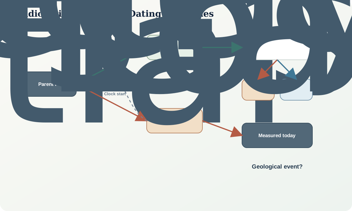
If each parent atom has a constant probability of decay per unit time, the number of parent atoms follows
$\frac{dN}{dt}=-\lambda N,$
with solution
$N=N_0e^{-\lambda t}.$
The half-life is the time for half the parent population to remain:
$t_{1/2}=\frac{\ln2}{\lambda}.$
Decay is statistical at the atom scale and effectively smooth for geological numbers of atoms. A decay constant is an external calibrated quantity with uncertainty and version. Changing an adopted constant can shift calculated ages coherently; it is not a random analytical effect.
A mineral becomes useful as a clock when parent and daughter inventories can be related to an event and later exchange is sufficiently constrained. Crystallisation, cooling, recrystallisation, precipitation or alteration may establish the relevant boundary. Different domains in one grain can start or reset at different times.
Parent-daughter equations and initial components
The radiogenic daughter accumulated since time zero is
$D^*=P(e^{\lambda t}-1),$
where P is the parent remaining today under this convention. If total daughter D includes an initial non-radiogenic component D_0,
$D=D_0+P(e^{\lambda t}-1).$
Solving a single parent-daughter pair requires knowledge or correction of D_0. Many systems use ratios to a stable non-radiogenic isotope to reduce concentration and instrument-yield dependence. The denominator isotope must be appropriate and its own behaviour understood.
The simple age is
$t=\frac{1}{\lambda}\ln\left(1+\frac{D^*}{P}\right).$
This equation assumes the measured parent and radiogenic daughter belong to the same reservoir, the system boundary is appropriate, and later gain or loss has been absent or corrected. An age can be mathematically exact for the supplied ratios yet geologically meaningless if these assumptions fail.
Isochrons, concordance and internal tests
An isochron uses several co-genetic reservoirs with a common initial daughter ratio and different parent/stable-isotope ratios. In generic form,
$\left(\frac{D}{S}\right)_{now} =\left(\frac{D}{S}\right)_0 +\left(\frac{P}{S}\right)_{now}(e^{\lambda t}-1).$
The slope gives e^{\lambda t}-1 and the intercept estimates the initial ratio. Scatter beyond analytical covariance may indicate geological heterogeneity, open-system behaviour, mixed ages or underestimated uncertainty. A line can also be a mixing array; petrographic and compositional evidence must test co-genesis and age meaning.
Some parent-daughter schemes provide two related decay pathways or ratio relations. Concordance between them offers an internal test, while discordance can record loss, inheritance or mixing. A discordant array can carry chronological information only under an appropriate disturbance model. Forcing discordant analyses into one weighted mean destroys that information.
Initial disequilibrium matters when intermediate daughters were not in secular equilibrium at clock start. Common or non-radiogenic daughter corrections, blank, tracer calibration and mass-fractionation corrections may also be needed. Each correction adds inputs and covariance that belong in the uncertainty model.
Sampling and measurement design
Choose material according to event and closure behaviour. A whole rock may average source components; a mineral separate may mix grains; a spot can isolate a zone but sample inclusions, cracks or multiple depth domains. Image grains before analysis and record cores, rims, overgrowths, alteration and defects. Relative-age textures guide which analyses may be pooled.
Preserve sample preparation, mineral separation, dissolution or ablation domain, blank, tracer or calibration version, interference corrections, mass fractionation, common-component treatment and raw ratio covariance. Reference materials monitor bias but do not make an unknown sample geologically closed.
Replicate measurements of one solution test measurement repeatability. Separate dissolutions test preparation and heterogeneity at a larger support. Multiple spots test domain variation but are not technical replicates. Report which level each uncertainty describes.
Worked synthetic examples
Half-life reasoning. A synthetic parent population has 25% of its initial atoms remaining. Since 0.25=(1/2)^2, two half-lives have elapsed. If the illustrative half-life is 1.25 Ga, the elapsed time is 2.50 Ga. The arithmetic does not identify when a mineral closed or whether parent or daughter was exchanged.
Parent-daughter calculation. Suppose corrected synthetic ratios give D^*/P=0.50 and the illustrative decay constant is 1.00\times10^{-10}\ \mathrm{a^{-1}}. Then
$t=\frac{\ln(1.50)}{1.00\times10^{-10}} =4.05\times10^9\ \mathrm{a}.$
If 10% of the daughter was lost, the observed ratio would be lower and the apparent age younger. If an unrecognised initial daughter was included in D^*, the apparent age would be older. Direction depends on what moved and how correction was defined.
Isochron slope. For a synthetic slope m=0.050 and \lambda=1.42\times10^{-11}\ \mathrm{a^{-1}},
$t=\frac{\ln(1+m)}{\lambda}=3.44\ \mathrm{Ga}.$
This value becomes an event age only if the samples were co-genetic, shared an initial ratio and remained appropriate reservoirs. Intercept, residuals, covariance and petrography are part of the result.
Interpretation workflow and uncertainty
- State the geological event to be tested before selecting material.
- Identify parent and daughter hosts, initial-component problem and likely exchange pathways.
- Map analytical domains to textures and relative-age relations.
- Apply corrections with recorded constants, reference materials and covariance.
- Calculate dates and internal consistency tests without premature rejection.
- Examine discordance, residuals and age populations against domain evidence.
- Separate analytical uncertainty from calibration, decay constant and geological scatter.
- Test inheritance, mixing, loss, gain, disequilibrium and resetting alternatives.
- Assign an event only where the evidence supports the clock boundary.
Failure modes
Common failures include assuming zero initial daughter, ignoring common components, treating all spots as equivalent replicates, using a weighted mean when scatter is geological, rejecting discordant analyses solely because they are inconvenient, and reporting an analytical date as a crystallisation age without texture. Another is comparing ages calculated with different constants or calibration versions as if they were on one scale.
Uncertainty has correlated components. A tracer or reference value may shift all analyses together; counting statistics may vary independently; common-component correction can correlate ratios within an analysis; and geological heterogeneity is not measurement error. Preserve covariance and state what is included in each quoted uncertainty.
Practice and review
- Derive the half-life relation from the decay equation.
- Calculate ages for
D^*/P=0.1,0.5and2.0using a supplied synthetic decay constant. - Show qualitatively how daughter loss, parent loss and inherited daughter affect an apparent age.
- Construct a five-point synthetic isochron with a common intercept, then perturb one point to represent alteration.
- Design an imaging and sampling plan for a grain with inherited core, igneous rim and later fracture alteration.
For the completion exercise, review a synthetic ratio table containing common-component correction, covariance and two textural domains. Calculate dates, inspect an isochron or concordance relation, retain rejected points with reasons, and state which event interpretations remain defensible.
Sources and further reading
- Steiger and Jäger, Convention on decay constants and isotopic age reporting90060-7), foundation for comparable constants and age conventions.
- Wetherill, Discordant uranium-lead ages, basis for interpreting concordant and discordant U-Pb relations.
- Horstwood and co-authors, Community-derived standards for LA-ICP-MS U-Th-Pb geochronology, measurement, uncertainty and reporting framework.
- McLean and co-authors, An algorithm for U-Pb isotope dilution data reduction and uncertainty propagation, transparent ratio reduction and covariance treatment.
- Renne and co-authors, Joint determination of potassium decay constants, calibrated constants and implications for age accuracy.