B5 · Publication Volume 10
Integrating Geochemical Evidence
whole-rock chemistry, mineral chemistry, isotopes and geological context
Learning goals
After this lesson, you should be able to integrate field relations, petrography, mineral chemistry, whole-rock compositions, aqueous or stable-isotope data and geochronology without treating them as independent votes. You should be able to build an evidence graph, audit compositional transformations, separate source-process-time hypotheses, and define a decision boundary for a geological conclusion.
Integration is not the act of placing many plots beside one another. It is the construction of a causal and temporal model in which each observation has a sampling support, each transformation has a declared equation, and each inference has alternatives. Contradictions are retained because they locate missing processes or mixed domains.
Evidence graph from object to event
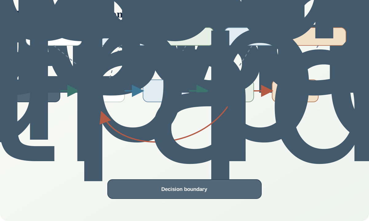
Represent the project as a graph. Object nodes are outcrops, intervals, grains, growth zones, veins and waters. Measurement nodes are observations, images, concentrations and isotope ratios. Transformation nodes include blank correction, normalisation, log-ratios, mass balance, speciation and date calculation. Model nodes represent mixing, reaction, fractionation, diffusion and decay. Event nodes represent formation, alteration, deformation, cooling or resetting.
Edges must have verbs: sampled from, measured by, corrected with, calculated from, supports, contradicts or cross-cuts. A direct field relation should not be given the same logical status as a regional analogy. Every event claim should be traceable backwards to objects and forward to predictions.
Evidence is not independent merely because it comes from different columns. Mineral chemistry and whole-rock chemistry may share the same sample; an age and trace-element pattern may come from the same spot; several isotope ratios may share one correction. Model shared uncertainty and provenance to avoid false confidence from double counting.
Compositional transformations and comparability
Geochemical tables combine different bases: weight percent oxides, mg/kg elements, molar ratios, isotope ratios and censored values. Convert only with documented formula masses, valence and basis. Preserve the original fields. A derived normalised table must retain its denominator and missing-data rule.
Closed compositions carry relative information. For positive components x_i, an additive log-ratio relative to denominator x_D is
$alr_i=\ln\left(\frac{x_i}{x_D}\right).$
A centred log-ratio compares each component with the geometric mean, while an isometric log-ratio uses orthonormal balances. The chosen coordinates should express a geological contrast and must handle zeros or detection limits explicitly. Replacing every censored value with one arbitrary fraction of detection limit can create artificial clusters.
Classification and discrimination diagrams have compositional, calibration and geological domains. They do not convert altered rock into a primary melt or mixed sediment into a source fingerprint. Before plotting, test alteration, cumulate character, grain-size effects and analytical comparability. Use diagrams as conditional evidence beside petrography and mass balance.
Spatial and temporal integration
Locations, depths and domains determine whether measurements can be combined. A metre-scale alteration front, a kilometre-scale source region and a micron-scale age domain answer different questions. Carry support and positional uncertainty into maps and sections. Interpolation should not cross geological boundaries merely because points are close in Euclidean distance.
Relative time constrains numerical time. Cross-cutting, overgrowth and replacement establish order before age calculation. A numerical date that violates a secure relation signals mixed domain, resetting, incorrect event assignment or an erroneous field model. Do not repair the conflict by silently relabelling the older observation.
Build event tables with columns for observed relation, dated domain, date result, uncertainty, interpretation and alternative. A regional correlation should remain a hypothesis unless material continuity, stratigraphy, chemistry or age supports it. Similar compositions can recur, and similar ages can represent different processes.
Causal models and competing hypotheses
Write at least two process models. For example, an element enrichment could reflect source addition, fluid transfer, residual concentration, mineral sorting or denominator loss. Each model predicts mineral hosts, complementary depletion, spatial gradients, isotope effects and timing. Design tests around predictions that differ.
A prior–likelihood–posterior framing can make evidence updating explicit, but numerical probabilities are not required when prior and likelihood information are weak. A qualitative evidence matrix can record whether each observation is expected, possible or contradictory under each model. Avoid counting correlated observations as independent likelihood multipliers.
Model complexity should be earned. A two-component mixing model is preferable to a five-reservoir narrative until residual structure demands more. Conversely, forcing a simple line through demonstrably multi-stage domains is not parsimony; it is loss of evidence.
The conclusion must contain a decision boundary. State where and under what conditions the model may be used, which samples are excluded and why, and what uncertainty prevents extension. A transferable tutorial result is a method and boundary, not a claim about a named property or organisation.
Reproducibility, reference data and review
Store stable identifiers for objects, samples, preparations, analyses, reference materials and derived datasets. Use controlled units and qualifiers. Record versions of thermodynamic databases, decay constants, reference compositions, classification boundaries and code. Derived plots should be rebuildable from immutable inputs.
Reference materials have purposes and matrices. A reference value is not a universal truth independent of method, and a material suitable for one element range may not validate another. Report blanks, duplicates and reference results with acceptance criteria. Quality-control failure must remain visible and prevent interpretation until resolved.
Independent review should be able to traverse the evidence graph, reproduce key calculations and challenge event assignments. Publication on a website does not constitute scientific review. Record authorship or review of a specific analysis only in its real project provenance; do not assign any company or person a relationship to this general tutorial.
Worked synthetic integration case
An invented traverse crosses an unaltered igneous unit, a fracture-centred alteration zone and a late vein. The synthetic data include twelve whole-rock samples, mineral maps from four samples, paired stable-isotope analyses and dated cores, rims and vein minerals.
Whole-rock components A, B and C change from 50:30:20 outside the zone to 40:40:20 inside. Raw percentages suggest A loss and B gain. Using C as a log-ratio denominator,
$\ln(A/C):\ \ln(50/20)=0.916\rightarrow\ln(40/20)=0.693,$
$\ln(B/C):\ \ln(30/20)=0.405\rightarrow\ln(40/20)=0.693.$
Mineral maps show destruction of A-bearing feldspar and growth of a B-bearing alteration phase, while C resides in resistant accessory grains. An immobile-reference balance with two candidate references supports moderate A loss and B addition but gives a wider range where accessory grains are mechanically concentrated.
Stable-isotope values shift only in replacement domains, not in unaltered cores. Dates define an old core population, a coherent igneous rim population and a younger vein population; two fracture-adjacent rims are partially reset. Cross-cutting shows the vein postdates alteration in one exposure but occupies the same pathway elsewhere.
The preferred model is: igneous crystallisation recorded by rims; later fluid-rock replacement focused by fractures; vein precipitation during or after the late part of fluid flow; and local resetting near permeable fractures. An alternative is two fluid events, because the cross-cutting relation and isotope shift are not identical everywhere. The decision boundary excludes mechanically sorted surface samples and mixed ablation domains. No economic, organisational or site-specific claim is made.
Completion workflow and review
- Inventory objects, support, units, preparation and quality-control status.
- Separate raw, corrected, normalised and modelled fields.
- Build field and petrographic relative order before numerical integration.
- Check charge, mass and isotope-bearing amount balances.
- Use compositional transformations suited to the geological contrast.
- Link ages to imaged domains and compare systematic uncertainty.
- Construct at least two causal-event models and list discriminating predictions.
- Map applicability, exclusions and unresolved boundaries.
- Publish an evidence ledger, reproducible calculations and a concise conclusion.
Completion review asks:
- Can every result be traced to a real observation or an explicitly synthetic exercise?
- Are company and personal names absent from the tutorial except as bibliographic source identifiers?
- Are reference scale, constants, database versions and corrections recorded?
- Are analytical dates separated from interpreted events?
- Are contradictions and rejected analyses visible?
- Would another reviewer know what evidence could change the conclusion?
The final deliverable is a review of an age-and-geochemistry dataset that distinguishes measurements, dates, processes, events and uncertainty sources. A result passes only when the evidence graph remains auditable if the preferred geological narrative changes.
Sources and further reading
- Aitchison, The Statistical Analysis of Compositional Data, foundation for log-ratio analysis of closed geochemical compositions.
- Winchester and Floyd, Geochemical discrimination using immobile elements90057-2), influential classification approach whose domain assumptions must remain explicit.
- GeoReM geological and environmental reference-material database, traceable compilation of reference-material values.
- Jochum and Nohl, Reference values for geological reference materials, evaluated concentration data and uncertainty context.
- FAIR Guiding Principles for scientific data, framework for reusable, interoperable and reviewable evidence.