A4 · Publication Volume 5
Constructing a Section from a Map
projection, true thickness, apparent dip, topography and continuation of units
Learning objectives
After this lesson, you should be able to build a topographic profile, project observations to a section plane, calculate apparent dip, maintain thickness cautiously and distinguish constrained geometry from interpretive continuation.
A section is a testable model
A geological cross-section is a vertical or near-vertical slice along a declared trace. It combines surface topography, mapped contacts, orientation data and interpretive rules. Because most subsurface geometry is not directly observed, the section is a hypothesis constrained by evidence, not a photograph of the underground.
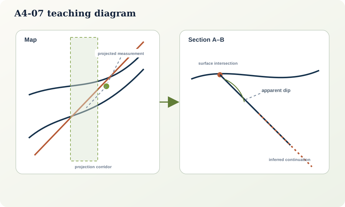
Declare the section frame
Every section needs:
- endpoints or a polyline trace with coordinates;
- view direction;
- horizontal and vertical scales;
- vertical exaggeration;
- elevation and horizontal references;
- projection width for off-line data; and
- a convention for observed, projected and inferred geometry.
A bent section can follow a valley or borehole fence but distorts azimuth relationships. Mark bends explicitly and do not measure apparent dip across them as though the plane were straight.
Step 1: topographic profile
Transfer contour crossings, spot heights and terrain breaks to the section baseline. If using a terrain model, record its resolution and date. Do not start geological lines until the profile and scales are verified.
Step 2: surface intersections
Mark where mapped contacts and faults cross the section trace. Preserve their location style: an inferred map contact remains inferred at the surface. If a broad contact corridor crosses the line, project the corridor rather than a single falsely exact point.
Step 3: project nearby observations
An orientation measured away from the section may be projected within a declared corridor if the structure is assumed continuous. Show the original point and projection distance. The farther the projection and the more heterogeneous the structure, the weaker the constraint.
For boreholes, project the actual trajectory, not only the collar. Clearly distinguish data on the plane from data projected onto it. A wide projection window can create impossible apparent correlations.
Step 4: convert true to apparent dip
Use the formula from Lesson A4-03. A bed striking 070° and dipping 35° southeast is crossed by a section trending 120°. The section is 50° from strike:
\psi=\arctan(\tan35^\circ\sin50^\circ)\approx28.2^\circ.
Plot approximately 28°, not 35°, before any correction for vertical exaggeration. With VE=2, the displayed angle \beta satisfies
\tan\beta=VE\tan\psi,
so the bed appears about 45.6° on the page. Label the exaggeration prominently.
Step 5: thickness and continuation
For parallel planar boundaries, true thickness is measured perpendicular to bedding. Outcrop width on a horizontal surface depends on dip; on sloping terrain it also depends on ground slope. In sections, do not preserve page-width as “constant thickness” when vertical exaggeration or obliquity changes geometry.
Maintaining thickness is a useful initial assumption for a laterally persistent sedimentary unit, but it is not universal. Units may thin, thicken, onlap, pinch out, be faulted or intruded. State the rule and stop lines where evidence no longer constrains them.
Step 6: balance relationships
Check that:
- units do not appear or vanish without an indicated termination;
- contacts do not cross unless geology permits it;
- relative-age relations agree with map and legend;
- faults displace appropriate units and do not displace younger cover unless mapped;
- folds have geometrically plausible limbs and hinges; and
- the section returns to all known surface intersections.
This is topological validation before detailed kinematic restoration.
Two valid alternatives
Two converging contacts beneath a covered valley may represent a fold closure, an erosional pinch-out or fault truncation. If no observation discriminates, draw alternatives or an uncertainty envelope. Choosing one smooth solution because it looks tidy is not geological evidence.
Practical investigation
Construct a section through the Open Ridge map with a 100 m projection corridor. Use three line styles: direct surface intersection, projected observation and inferred continuation. Then construct a second valid geometry beneath the covered valley. List one new station or borehole that would best distinguish them.
Common failure modes
- Omitting view direction or vertical exaggeration.
- Plotting true dip in an oblique section.
- Projecting distant observations without showing distance.
- Correlating borehole intervals by elevation alone.
- Extending contacts to the bottom of the page without evidence.
- Forcing constant thickness through faults or unconformities.
- Presenting one interpretation where several satisfy the map.
Mastery check
- Which seven frame declarations belong on a section?
- Why does map-contact uncertainty carry into the section?
- Calculate apparent dip for 45° true dip and a section 40° from strike.
- How does
VE=3change the displayed angle? - What observations could distinguish a fold closure from fault truncation?
Sources and further reading
- USGS, *Apparent Dip Calculator*: https://pubs.usgs.gov/publication/tm7C28/full
- USGS, *Digital Geologic Cross Sections*: https://pubs.usgs.gov/of/2005/1428/thoms/index.html
- FGDC, *Geologic Map Symbol Standard*: https://ngmdb.usgs.gov/fgdc_gds/geolsymstd/download.php