A4 · Publication Volume 5
Generalisation, Scale and Uncertainty
boundary width, resolution, extrapolation and the false precision of clean graphics
Learning objectives
After this lesson, you should be able to explain why map content changes with scale, distinguish simplification from uncertainty, audit false graphical precision and design representations that remain honest when zoomed or reused.
Selection is unavoidable
No map contains every observable feature. Generalisation selects, aggregates, simplifies, displaces or symbolises information so it remains legible for a purpose and scale. A smaller-scale map covers more area and therefore usually omits narrow units, short faults, local folds and station detail. Omission is not necessarily error, but the selection rule must be understood.
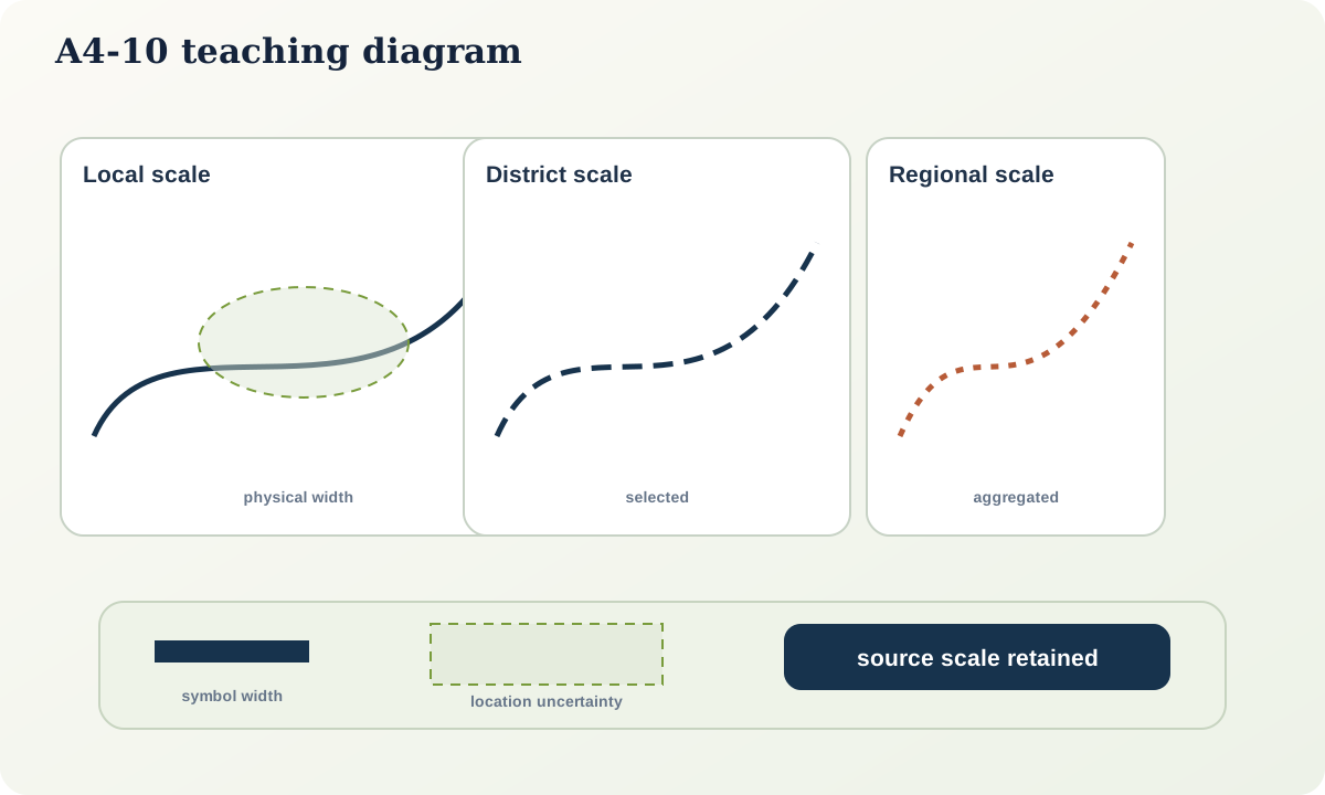
Four different widths
Do not confuse:
- physical boundary width — the actual transition or damage zone;
- locational uncertainty — where the selected boundary criterion may lie;
- symbol width — the graphic line on a map; and
- minimum mappable width — the narrowest feature represented as a polygon at that scale.
A 60 m alteration zone may have boundaries located to ±5 m but be shown by a 0.4 mm line at 1:250,000, whose ground width is 100 m. Alternatively, a sharp contact may be uncertain by 200 m. These cases need different descriptions.
Generalisation operations
- selection: retain features important to the map purpose;
- aggregation: combine several small bodies into a composite unit;
- collapse: represent a narrow polygon as a line or point;
- simplification: reduce vertices while preserving characteristic shape;
- smoothing: reduce angular noise;
- displacement: move symbols slightly to keep them legible; and
- classification: reduce the number of categories.
Each operation changes what can be measured from the display. Metadata should preserve source scale and transformation history.
Zoom does not restore detail
Enlarging a 1:250,000 source on screen does not make it a 1:10,000 observation. Vector lines remain sharp because they are mathematically rendered, not because their positions became more accurate. Interfaces should reveal source scale, resolution and confidence at every zoom and, where possible, substitute a more appropriate dataset rather than only enlarging symbols.
Quantifying an uncertainty corridor
If a contact is constrained at three stations with different location uncertainties, a constant-width buffer may be misleading. Interpolate an envelope that accounts for point accuracy, exposure density, terrain and geological complexity. Keep the centreline interpretation and confidence surface as separate data.
Uncertainty is not always symmetric. A contact below a cliff may be tightly constrained upslope but poorly constrained beneath colluvium downslope. Use an asymmetric corridor or categorical sectors.
A scale ladder
Prepare linked products rather than one map stretched across every decision:
- regional view: major terranes, basins and structures;
- district view: formations, intrusions and principal faults;
- local view: members, alteration zones and dense observations;
- station view: exposed surfaces, measurements and sample links.
Moving between levels requires rules for aggregation and provenance. A local interpretation should remain traceable to its observations; a regional line should reveal that it summarises many local segments.
Worked false-precision audit
A digitised historical contact has vertices every 2 m, displayed at 1:5,000. The source was traced from a 1:100,000 paper map with a 0.5 mm line. Its source symbol alone represented about 50 m, before registration and geological uncertainty. The dense vertices describe the digitising curve, not 2 m geological accuracy. Store source scale and uncertainty; simplify vertices if appropriate; do not advertise the coordinate spacing as accuracy.
Practical investigation
Create the same synthetic geology at 1:5,000, 1:25,000 and 1:250,000. For each scale, decide which units remain polygons, which collapse to lines, which aggregate and which observations disappear. Record the rule in a generalisation table. Then calculate ground-equivalent symbol widths.
Common failure modes
- Treating omitted detail as proof that a feature is absent.
- Confusing boundary width with locational uncertainty.
- Claiming improved accuracy after digitising or zooming.
- Buffering every line by one arbitrary distance.
- Simplifying geometry without preserving source provenance.
- Combining datasets of different scales without a hierarchy.
- Using a precise centreline where only an uncertainty zone is defensible.
Mastery check
- Name the four widths that must remain distinct.
- What changes when a polygon collapses to a line?
- Why are densely spaced vertices not evidence of accuracy?
- When should an uncertainty corridor be asymmetric?
- What provenance should follow a generalised regional boundary?
Sources and further reading
- USGS, *Generalization*: https://www.usgs.gov/centers/cegis/science/generalization
- USGS, *Field Description of Scientific and Locational Accuracy*: https://pubs.usgs.gov/of/2002/of02-370/soller1.html
- USGS, *Mining Information from Published Geologic Maps*: https://pubs.usgs.gov/of/1997/of97-269/collins.html