B4 · Publication Volume 9
Geomorphology, Remote Sensing and DEM Interpretation
landform metrics, drainage anomalies and resolution
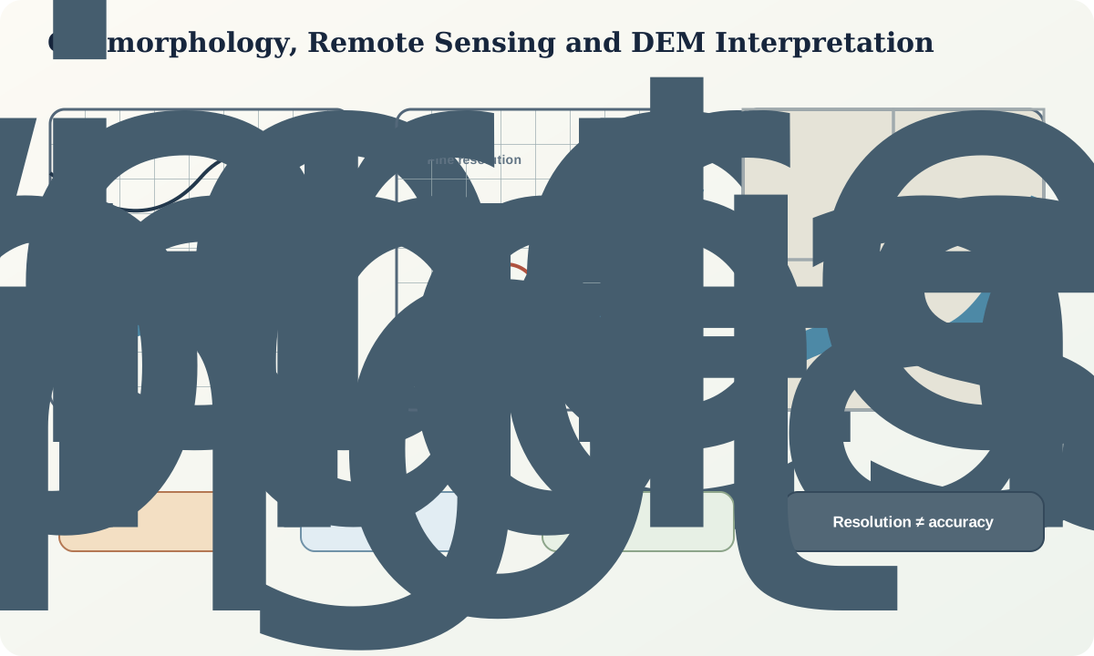
Learning objectives
After this lesson, you should be able to distinguish elevation models of surface and terrain; calculate slope, aspect and a relative-position metric; explain flow routing and drainage extraction conceptually; identify artefacts caused by void filling, vegetation, interpolation and projection; test interpretations at more than one resolution; and record a reproducible terrain-analysis chain without treating derived metrics as direct geological observations.
Start with a field problem
A shaded-relief image shows a linear valley, a circular depression and a sharp break in slope. Are they a fault-controlled drainage, a palaeochannel, a processing seam, a quarry, vegetation height, a sink created by data error or ordinary landform convergence? A visually striking line is evidence only after the elevation source, processing and ground relation are checked.
Remote sensing extends observation but changes support. A pixel averages or estimates a footprint; a digital surface can include vegetation and structures; an interpolated terrain can remove or invent depressions. Hillshade depends on illumination and can reverse apparent relief. Always return from image pattern to terrain quantity and then to field or independent evidence.
Core process model
A digital surface model represents the upper reflective surface, potentially including vegetation and structures. A digital terrain model aims to represent ground elevation after filtering. “DEM” is often used generically, so record the actual product definition. Essential metadata include horizontal and vertical reference systems, cell size, acquisition method and date, vertical accuracy, nodata treatment, filtering and resampling.
For gridded elevation z(x,y), local slope magnitude can be approximated from gradients:
\theta=\tan^{-1}\sqrt{\left(\frac{\partial z}{\partial x}\right)^2+\left(\frac{\partial z}{\partial y}\right)^2}.
Aspect is the downslope direction of the gradient and is unstable on nearly flat cells. Curvature measures changes in gradient and depends strongly on neighbourhood and noise. Topographic position compares a cell with a declared surrounding neighbourhood; the same location can be a local ridge at one scale and part of a regional valley at another.
Flow routing assigns downslope connections after handling flats and depressions. A depression may be real, such as a closed basin, or artefactual. Filling every sink can erase meaningful landforms; preserving every sink can fragment a drainage network. Channel initiation thresholds are model choices that change network density.
Remote-sensing reflectance or radar response may help map moisture, mineral or surface texture, but each sensor measures wavelength-specific interaction with the surface. Terrain, atmosphere, illumination, vegetation, grain size and moisture can confound geological interpretation. Derived classifications require independent validation.
Evidence and measurement
Inspect the elevation distribution, nodata mask, seam lines, striping, spikes, pits and relation to vegetation or infrastructure before deriving landforms. Compare contours and profiles with independent control points or a higher-quality local survey. Reproject using a suitable coordinate system before measuring horizontal distance or area; record all vertical transformations.
Calculate metrics at multiple resolutions and neighbourhood sizes. Preserve the unmodified source raster and each processing step. A drainage anomaly should be tested against geology, regolith, imagery, field observations and the unconditioned DEM. Separate automatically extracted channels from mapped watercourses and from inferred palaeodrainage.
Ground validation should sample both predicted positives and predicted negatives. If only obvious anomalies are visited, accuracy cannot be estimated. Record the exact feature tested, its scale and the observation that supports or contradicts the remote interpretation.
Worked example
In a synthetic 3-by-3 elevation window, the east–west elevation difference over 60 m is 6 m and the north–south difference is 3 m. Approximate gradients are 0.10 and 0.05. The slope is
\theta=\tan^{-1}\sqrt{0.10^2+0.05^2}=6.38^\circ.
If the same surface is resampled to a coarser grid, the maximum local difference may fall and the derived slope may be lower. This is not necessarily landscape change; it is a scale effect.
Now compare a circular depression in three products. It persists in the unconditioned terrain model, aligns with closed contours, contains fine sediment and has no processing seam: a real closed basin is plausible. If it appears only after filtering, follows a tile edge and disappears in independent elevation data, an artefact is more plausible. The conclusion comes from convergence of evidence, not shape alone.
Misinterpretations and uncertainty
Do not infer fault displacement from a straight valley without offset markers, structural measurements or subsurface evidence. Do not infer a crater, sinkhole or palaeochannel from circularity alone. Drainage alignment can reflect joints, bedding, slope, land use or algorithmic conditioning.
Resolution is not the same as accuracy. A small cell can interpolate noisy or biased measurements. Vertical error that is minor on steep terrain can dominate slope in a low-relief plain. Hillshade azimuth changes visibility, and vertical exaggeration distorts gradient. Report uncertainty and processing choices beside every terrain-derived boundary.
Practical investigation
Using an openly documented teaching DEM, preserve a source copy and create a processing log. Generate slope, aspect, two topographic-position scales and two drainage networks using different thresholds. Mark features that persist and those that appear only under one setting.
Choose one persistent and one unstable feature. Build geological, geomorphic and artefact hypotheses for each. Design a validation route containing positive and negative checks and specify the field evidence that would change the interpretation.
Mastery check
- How does a terrain model differ from a surface model?
- Why is aspect unstable on flat ground?
- What happens when all DEM depressions are filled automatically?
- Why must terrain metrics be tested at more than one scale?
- Which evidence turns a linear terrain pattern into a structural interpretation?
Sources and further reading
- High-resolution topography for understanding Earth surface processes, Tarolli, 2014.
- Effects of spatial resolution on slope and aspect, Grohmann, 2015.
- Flowline assessment of channel extent and type, Johnson and co-authors, 2023.
- Australian elevation data and digital elevation models, Geoscience Australia, official dataset guidance.