D2 · Publication Volume 18
Data Quality and Support
sampling quality, support, bias and the volume–variance relationship
Learning objectives
By the end of this lesson, the learner should be able to distinguish analytical quality from spatial representativity; define sample support in physical terms; check interval, coordinate, density and missing-value conventions; explain the volume–variance relationship; and decide whether data are fit for a specific estimation purpose.
Data quality is multidimensional. A precisely assayed sample can still be unrepresentative because of poor recovery, selective loss, clustering or an incorrect domain assignment. A coordinate may be numerically valid but referenced to the wrong grid. Fitness must be evaluated along the entire measurement chain.
Source register and data lineage
Create a register for collars, surveys, intervals, assays, density, geology, quality-control results and derived fields. Record identifiers, units, coordinate reference, vertical datum, sampling method, support dimensions, laboratory basis, detection limits, missing-value codes, version and transformation lineage. A numeric zero must never stand ambiguously for not sampled, below detection, absent material and true zero.
Use immutable source keys and preserve duplicates until their relationship is resolved. Corrections should produce a traceable state change rather than overwrite the original record. Derived coordinates, desurveyed traces, composites and coded domains must point back to the source rows used.
Interval, coordinate and geometry checks
For every hole, test collar uniqueness, survey order, depth monotonicity, maximum depth, interval order, negative lengths, overlaps, gaps and out-of-hole records. Compare downhole interval endpoints with the desurveyed trace and the adopted model extent. Plot collars, traces and samples in plan, section and three dimensions; tabular validity does not reveal a systematic grid shift or an inverted vertical axis.
Tolerance must have a physical basis. A tiny floating-point mismatch between adjacent intervals may be harmless; a short unsampled gap at a sharp boundary may materially change compositing. Store the original values and the tolerance-based interpretation separately.
Measurement quality and density basis
Review recovery, contamination controls, reference materials, blanks, duplicates, detection limits and laboratory changes before statistical transformation. Investigate failures by batch, time, material type and grade range. Do not average away a systematic bias. Quarantined data should remain visible with reason and decision status.
Density requires equal discipline. Record method, moisture condition, sample preparation, lithology, alteration, weathering and support. A single global density can create a larger tonnage error than a local grade difference. Compare density coverage with the geometry and classification volume, and prevent extrapolation into materials not represented by the measurement method.
Support and comparability
Support is the volume, mass, length and orientation over which a value is averaged. For an interval with length l_i, cross-sectional area A_i and effective recovery r_i, a conceptual physical support is proportional to l_iA_ir_i, although the reported grade may not explicitly incorporate all three. Two samples at the same midpoint are not equivalent if their lengths or collection methods differ.
Before comparing distributions, align or explicitly model support. Length-weighted means are appropriate for additive grades over compatible intervals:
\bar z_L=\frac{\sum_i l_i z_i}{\sum_i l_i}.
Mass weighting may be needed when density varies materially. Never use an arithmetic mean of unequal intervals as a substitute for a support-aware calculation.
Volume–variance relationship
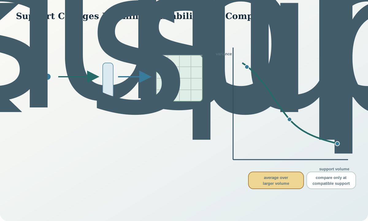
As support increases, local high and low values are averaged. For an additive variable in a stable domain, the mean may remain approximately constant while variance generally decreases. Consequently, a sample histogram cannot be treated as the expected block histogram. The amount of material above a cut-off depends on block size, spatial continuity and selectivity.
This relationship is not a licence to force an estimated histogram to an arbitrary target. Trends, boundary mixing, non-additive variables and biased sampling can violate simple expectations. Use support-change calculations, sensitivity studies or simulation with clearly stated assumptions.
Synthetic worked example
The synthetic dataset contains intervals from 0.4 to 3.6\,\mathrm{m}. An unweighted assay mean is 1.18 units, while the length-weighted mean is 1.07. Investigation shows that short intervals were preferentially selected around visible high-grade material. A density table also uses two moisture bases. The team separates the bases, corrects the unit metadata and calculates domain-specific coverage.
After two-metre compositing, the variance falls from 2.46 to 1.71 square units while the length-weighted mean changes by less than 0.5\%. A ten-metre block-support sensitivity predicts further smoothing. The result is recorded as a support effect, not evidence that the high assays were wrong.
Practice and review checklist
- Define the physical and numerical support of every primary variable.
- Reconcile missing, zero, below-detection and not-applicable codes.
- Compare arithmetic, length-weighted and, where justified, mass-weighted means.
- Map recovery, quality-control failures, density coverage and support by domain.
- Test whether a change in support preserves mean and changes variance in a plausible direction.
Decision record and integration
The data-readiness record should list accepted, corrected, quarantined and excluded rows; the reason for each rule; unresolved risks; support definitions; density bases; and the input version frozen for estimation. It should state which domains and confidence categories each data type may support.
Compositing, declustering, variography and estimation must use this frozen population or document a new gate. If a later correction changes a material statistic, every dependent result should be invalidated through the workflow graph.
Sources
- Mineral-resource and mineral-reserve estimation best-practice guidelines, details data verification, sampling, density, database integrity and fitness considerations before estimation.
- Change of support and the volume–variance relation, explains why variability changes between sample and selective-block support.
- GeoSciML 4.1, provides a standards-based logical model for geological observations, boreholes and feature relationships.
- Compositing and regularization of drillhole data for geostatistical resource estimation, documents local and global bias that can arise when support and gaps are handled poorly.