D2 · Publication Volume 18

Exploratory Data Analysis

distributions, outliers, domains and relationships

Learning objectives

By the end of this lesson, the learner should be able to build a domain-aware exploratory analysis; interpret robust and conventional summaries; distinguish tail behaviour from error; compare groups without ignoring support or spatial location; and turn statistical observations into testable geological questions.

Exploratory analysis is not a search for a preferred distribution. Its purpose is to expose structure, mixtures, trends, support effects, data-quality issues and assumptions that later methods must address.

Analysis population and audit table

Define the population before plotting. Record domain, variable, data type, support, date range, detection-limit treatment, recovery filter, capping state and transformation. A histogram labelled only with a variable name is not reproducible. Include counts and total support so a group with many short intervals is not mistaken for a larger physical population.

Create an audit table showing the population after each filter. Unexpected changes in count, total length, weighted mean or high-grade contribution often reveal a join error or an overly broad exclusion rule.

Distribution views and robust summaries

Use complementary views: histogram, cumulative distribution, box plot, quantile plot and ranked contribution. Report count, minimum, maximum, quantiles, mean, median, variance, standard deviation, coefficient of variation and robust spread. For positive skewed data, the mean and variance remain important for metal accounting, but median and quantiles show the typical observation without being dominated by the tail.

Histogram shape depends on bin width and axis scale. Always inspect the same population on linear and, where values are positive, logarithmic axes. A smooth curve can hide small subpopulations; a noisy histogram can create false modes. Keep the individual high values visible.

Group comparisons and domain testing

Compare geology, alteration, weathering, orientation, drilling phase, sample type and spatial sector. Use side-by-side distributions and quantile–quantile comparisons, then map the differences. Statistical separation supports a question about domains but does not define a boundary by itself. Conversely, overlapping distributions do not disprove a geologically meaningful boundary if continuity differs.

When groups have different supports or sampling density, align them before interpreting mean differences. A densely drilled high-grade core can dominate an unweighted global histogram. Report both raw and declustered sensitivities where preferential sampling is plausible.

Relationships, trends and multivariate checks

Scatter plots, rank correlations and conditional summaries can reveal density–grade, element–element or recovery–grade relationships. Mark detection limits and censored values rather than treating them as ordinary zeros. Use colour or facets for domains; a pooled correlation may be created entirely by differences between groups.

Plot values against easting, northing, elevation, depth and geological coordinates. A trend can be real, a drilling-phase effect or a boundary mixture. Later stationary methods require either a defensible stable domain or an explicit treatment of trend.

Outliers as questions

An extreme value can be an error, a correct rare observation, a support anomaly or evidence of a separate geological process. Investigate source certificates, units, duplicates, recovery, neighbours and geological context. Do not delete a value because it violates a convenient distributional model.

Separate detection from treatment. Flag candidate extremes with transparent criteria, then decide whether to correct, exclude, cap, restrict spatial influence, model separately or retain. The effect on contained quantity and local estimates belongs in a later sensitivity study.

Synthetic worked example

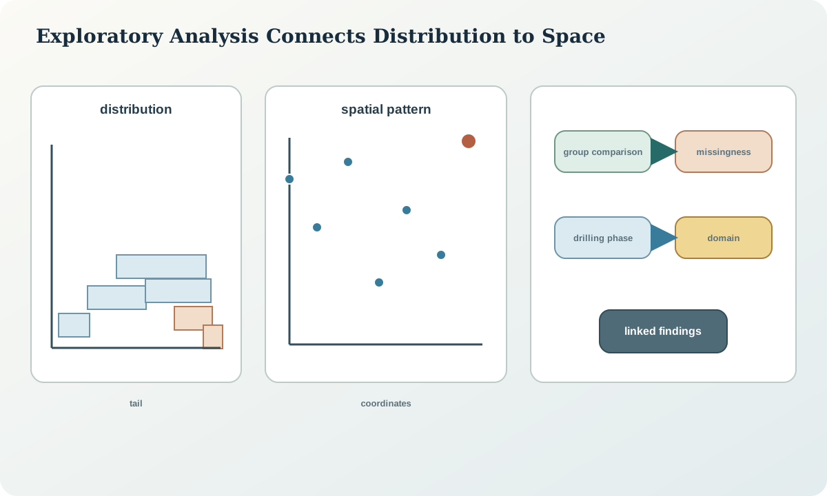
In the synthetic central domain, 63% of samples lie in 28% of the volume. The raw mean is 1.34, median 0.62 and coefficient of variation 1.9. A log-scale histogram shows a continuous tail rather than a clean second mode. Five high values contribute 17% of the total sample metal accumulation.

Colouring by drilling phase shows that three high values come from one campaign, but certificate and duplicate checks pass. Mapping shows they follow a narrow fold limb. The decision is to retain them for compositing, flag the structural subzone and test capping and restricted influence later. No new domain is created solely from the histogram.

Practice and review checklist

• Produce an analysis-population statement and filter audit table.
• View each important variable with at least four complementary distribution plots.
• Compare raw, support-weighted and declustered summaries by domain.
• Map every apparent group difference or trend before interpreting it.
• Create an extreme-value investigation register without automatically deleting observations.

Decision record and integration

The exploratory record should state which populations appear stable, which trends or mixtures need modelling, which values require investigation and which transformations are proposed. Preserve plots with data-version, filter and support metadata.

The outputs guide composite length, declustering direction, variogram domains, anisotropy and extreme-value tests. They do not by themselves authorise any of those decisions.

Sources

• Exploratory Data Analysis, gives an official framework for graphical investigation, assumptions and complementary diagnostics.
• Histogram, explains binning, normalisation and the distribution features a histogram can reveal.
• Detection of outliers, separates outlier identification, investigation and robust accommodation.
• The decision of stationarity, connects domain and trend decisions to the assumptions used in spatial estimation.