D2 · Publication Volume 18
Declustering
preferential sampling, weights and representativity
Learning objectives
By the end of this lesson, the learner should be able to recognise preferential sampling; explain why a raw sample mean may not represent a spatial domain; calculate and review declustering weights; select dimensionality and cell-size sensitivities; and state what declustering can and cannot correct.
Drilling is rarely located by random sampling. Dense follow-up commonly targets interesting areas, access corridors or uncertain contacts. The resulting data may be excellent for local estimation while giving a biased picture of the whole domain if every sample receives equal global weight.
Preferential sampling and representativity
Plot sample density and value together. Preferential sampling is suggested when high- or low-value areas have systematically different spacing. Compare drilling phases, sectors and domain volumes. A clustered dataset is not automatically biased: clustering matters when placement relates to the variable or to a geological feature associated with it.
Define the estimand. A global domain mean, a local block estimate and a sample histogram answer different questions. Declustering primarily addresses representative global distributions or proportions; local estimators already account for location through their neighbourhood and weights.
Cell declustering principle
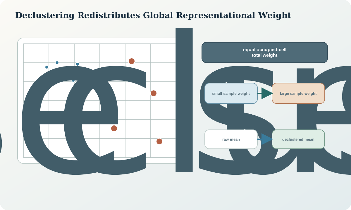
Partition the domain into equal-volume cells. Give each occupied cell equal total weight, then divide that cell weight among the samples it contains. If cell j contains n_j samples and there are N_o occupied cells, an unnormalised sample weight is proportional to 1/n_j; normalised weights satisfy
w_i=\frac{1/n_{j(i)}}{\sum_{k=1}^{n}1/n_{j(k)}} , \qquad \sum_i w_i=1.
The declustered mean is \bar z_w=\sum_iw_iz_i. The result depends on cell size and grid origin, so neither may be hidden.
Dimensionality, coordinates and boundaries
Use the dimensions in which sampling is preferential. A tabular domain intersected by holes approximately perpendicular to its plane may require declustering in geological two-dimensional coordinates. A thick or irregular body may require three dimensions. Declustering in map coordinates can be misleading if the domain is folded or rotated.
Cells cut by boundaries can overweight small occupied fragments. Test domain-specific grids, geological coordinates and boundary sensitivities. Samples from different stationary populations should not share declustering weights merely because they occupy the same spatial cell.
Parameter selection and stability
Test a range of cell sizes from dense spacing toward sparse spacing and multiple grid origins. Plot declustered mean, quantiles and effective sample size against cell size. Seek a stable region that is physically plausible, not the most favourable minimum or maximum. Report the raw result alongside the sensitivity envelope.
An effective sample size diagnostic is
n_{\mathrm{eff}}=\frac{1}{\sum_i w_i^2}.
A small value signals that a few sparse samples control the declustered distribution. That result may be mathematically consistent but too fragile for a confident global inference.
Limits and alternative evidence
Declustering cannot invent observations in unsampled space, correct analytical bias, repair wrong domains or remove geological trend. It assumes the chosen cells and coordinates provide a meaningful approximation to spatial representation. When sparse regions differ systematically, stratified estimates, trend models or explicit scenarios may be more honest.
Compare declustering with polygonal or nearest-area weighting, equal weighting by drillhole, and volume-stratified summaries where appropriate. Agreement increases confidence; disagreement identifies a representativity risk that should propagate into classification and uncertainty.
Synthetic worked example
The raw mean of the central domain is 1.34. A density map shows close-spaced drilling around the folded high-grade core and sparse drilling on the margins. Three-dimensional cell tests from 25 to 150\,\mathrm{m} yield declustered means from 1.02 to 1.16, with a plateau near 1.09 for cells comparable to sparse spacing.
Four grid origins produce a 1.06–1.12 range at the adopted cell size. The result is recorded as a representative-distribution sensitivity, not used to rescale individual data. A marginal sector with only three holes remains an explicit uncertainty even though declustering gives it higher weight.
Practice and review checklist
- Map data spacing and values by drilling phase and domain.
- State the estimand before applying any declustering method.
- Test two- and three-dimensional coordinates where geology warrants it.
- Plot mean, quantiles, effective sample size and origin sensitivity across cell sizes.
- Carry the raw, adopted and sensitivity distributions into later validation.
Decision record and integration
The declustering record should contain population, coordinates, dimensionality, cell sizes, origins, weights, diagnostic plots, selected range and limitations. Preserve weights as a separate field keyed to the composite version.
Use the result to inform global distribution, tail contribution, simulation inputs and validation targets. Do not apply declustering weights directly inside an estimator unless that specific method and purpose have been justified.
Sources
- Cell declustering parameter selection, explains cell weights, dimensionality, grid origins and practical parameter selection.
- Mineral-resource and mineral-reserve estimation best-practice guidelines, requires representative statistics and documented treatment of clustered data.
- Exploratory Data Analysis, provides the statistical context for examining sampling patterns, assumptions and distribution sensitivity.
- Change of support and the volume–variance relation, separates spatial representativity from the distinct effect of measurement and block support.