D2 · Publication Volume 18
Capping and Extreme Values
high-grade tails, risk and sensitivity
Learning objectives
By the end of this lesson, the learner should be able to investigate extreme values; distinguish error correction from high-grade management; quantify metal contribution and spatial influence; compare capping, restricted influence and separate modelling; and document sensitivity without presenting a subjective threshold as fact.
Extreme values matter because grades are additive and a small number of samples can control contained quantity. They must be taken seriously rather than automatically accepted or removed. The decision combines data quality, support, geology, spatial continuity and consequence.
Investigation before treatment
Trace each candidate value to source, units, analytical method, detection range, recovery, duplicate evidence and geological context. Check neighbouring intervals, nearby holes and structural position. Re-assay or alternative-method evidence may correct a measurement, but an unverified suspicion is not a correction.
Plot ranked values, cumulative metal contribution, linear and log probability views, spatial location and local neighbourhood. Examine extremes before and after compositing because averaging can hide a short high value or create a high composite from several moderate intervals.
Tail contribution and spatial continuity
For equal-support composites, a simple global contribution of values exceeding threshold c is
R(c)=\frac{\sum_i z_i\,I(z_i>c)}{\sum_i z_i}.
With unequal support, use length or justified mass weights. A high contribution does not prove the values are wrong; it shows that the estimate is sensitive to how they are extended.
Compare high-indicator and high-grade continuity with the main population. Extreme values often have shorter continuity than moderate grades. A single variogram dominated by the tail can transmit isolated values too far.
Capping and its accounting
Capping replaces z_i above a threshold c with z_i'=\min(z_i,c). Always retain both fields. Report the removed accumulation and the effect on raw and declustered means. Select candidate thresholds from multiple lines of evidence, then test them through estimation and validation.
A cap is not an outlier detector and should not be chosen merely where a probability plot bends. It is a model of limited high-grade contribution. If used, the geological and spatial rationale must accompany the numerical threshold.
Restricted influence and separate models
Alternatives include a smaller search for extreme values, a maximum number of high samples per estimate, indicator-based treatment, separate high-grade domains, residual models and conditional simulation. Each makes different assumptions. Restricted influence controls spatial reach while retaining the sample value; capping changes the value itself.
Avoid double treatment unless explicitly evaluated. Capping a value and then applying a severe high-grade restriction can understate contribution. Conversely, creating a hard high-grade domain from a few samples can exaggerate continuity.
Sensitivity and decision consequence
Run uncapped and several capped or restricted cases with identical other parameters. Compare domain mean, block mean, contained quantity, grade–tonnage curves, local high-grade volumes and swath plots. Map the difference. A small global change can hide a material local effect.
Classification should reflect sensitivity. A volume whose quantity changes materially across plausible treatments may require lower confidence, additional sampling or scenario reporting rather than a single precise answer.
Synthetic worked example
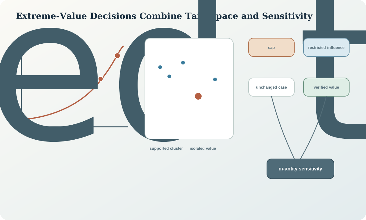
Five composites above 8.0 units contribute 17% of raw accumulation but 11% after declustering. Two are supported by adjacent high intervals along the fold limb; three are isolated. Candidate caps at 8, 10 and 14 units change total estimated quantity by -9.1\%, -5.4\% and -2.2\% relative to uncapped estimation.
A restricted-influence case retains all values but limits composites above 10 units to half the main search range. It produces a total between the 10 and 14 cap cases and removes a local high-grade halo around an isolated sample. The adopted teaching case uses the restriction, while all four alternatives remain in the uncertainty package.
Practice and review checklist
- Trace every candidate extreme to source and geological context.
- Calculate raw, support-weighted and declustered tail contribution.
- Compare continuity of the high indicator with continuity of the main variable.
- Run at least three plausible treatments with all other parameters fixed.
- Map local quantity differences and link material sensitivity to classification.
Decision record and integration
The extreme-value record should include candidate identification, verification evidence, thresholds, original and treated fields, accumulation removed, spatial-influence rules, estimation sensitivities, reviewers' rationale and unresolved uncertainty.
Variograms and estimates must identify which field they use. A later change in treatment invalidates the affected continuity model, estimate, validation and grade–tonnage outputs.
Sources
- A simulation approach to calibrate outlier capping, presents spatial and quantity-based sensitivity for choosing high-grade treatment.
- Detection of outliers, stresses investigation and distinguishes erroneous observations from scientifically important extremes.
- Dealing with high-grade data in resource estimation, reviews high-grade diagnostics, spatial restriction, capping and validation consequences.
- Mineral-resource and mineral-reserve estimation best-practice guidelines, requires transparent treatment and sensitivity of values that materially affect an estimate.