D2 · Publication Volume 18
Spatial Continuity and Variograms
nugget, sill, range, anisotropy and experimental variograms
Learning objectives
By the end of this lesson, the learner should be able to calculate an experimental semivariogram; select lag tolerances and directions; interpret nugget, nested structures, sill, range and anisotropy; fit a permissible model; and assess whether the available pairs support the continuity claimed.
A variogram describes average squared difference as a function of separation. It is not a picture of a geological object and does not prove stationarity. It translates a domain and support hypothesis into a quantitative continuity model used by kriging, support change and simulation.
Experimental semivariogram
For pairs separated approximately by vector \mathbf{h},
\hat\gamma(\mathbf{h})=\frac{1}{2N(\mathbf{h})}\sum_{i=1}^{N(\mathbf{h})}[z(\mathbf{u}_i)-z(\mathbf{u}_i+\mathbf{h})]^2.
Record pair count, mean lag, lag spread, mean pair value and contributing holes. A semivariance point without its pair support is easy to overinterpret. Avoid pairs formed by duplicated composites from one original assay.
Lag design and pair diagnostics
Choose lag distance from data spacing and the scale of expected continuity. Tolerances that are too narrow yield unstable points; tolerances that are too wide mix distances and directions. Limit maximum lag relative to domain extent, because long-lag pairs are few and may compare different trends.
Inspect variogram maps, pair-location plots and downhole variograms. The downhole direction helps separate short-scale variability and measurement effects from broader three-dimensional continuity. Test robustness to high values, composite length and domain changes.
Directional continuity and anisotropy
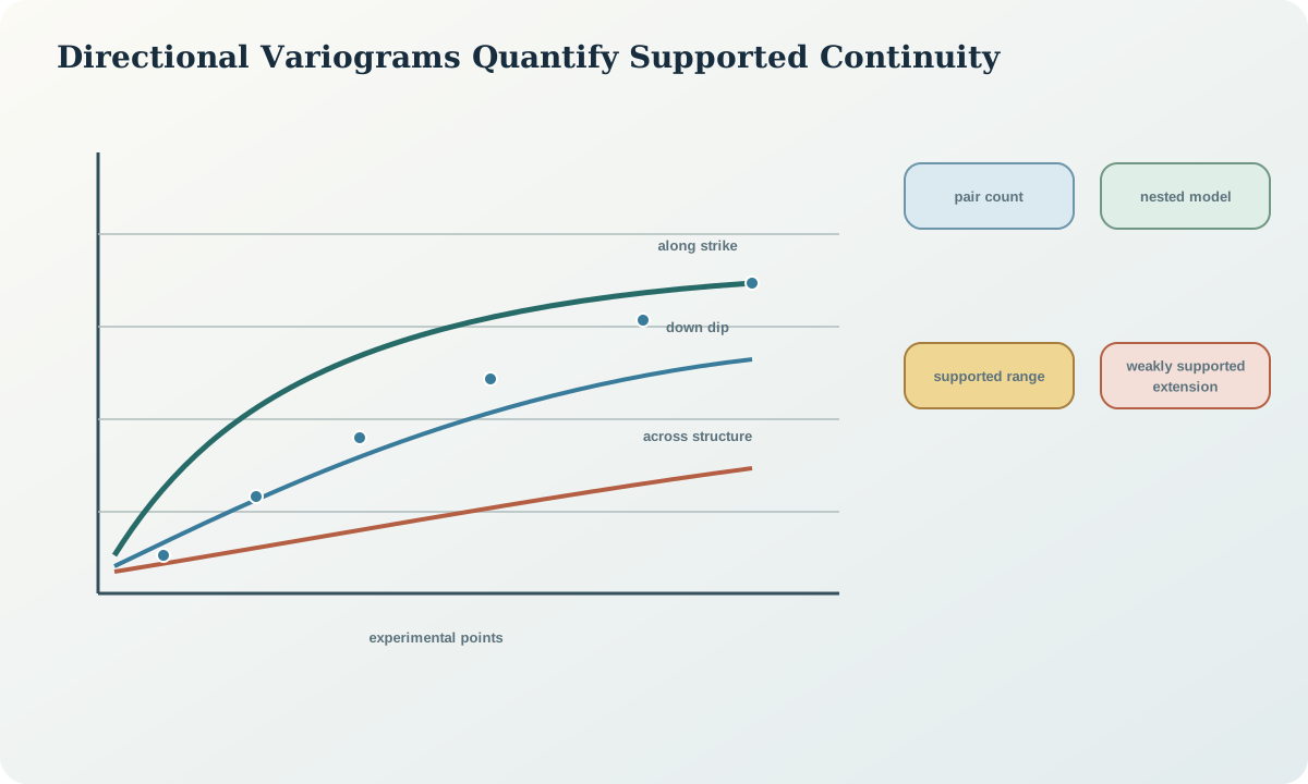
Define directions in geological coordinates where possible: along strike, down dip and normal to the principal fabric. A directional cone needs azimuth, dip, angular tolerances and bandwidth. Rotate directions systematically rather than selecting only the smoothest plots.
Geometric anisotropy has similar sill but different ranges. Zonal behaviour may show different directional sills or a range beyond the domain. Nested structures can represent continuity at more than one scale. The adopted axes should be compatible with geological interpretation and not merely a mathematical fit.
Nugget, sill, range and model fitting
The nugget represents variability below sample spacing plus measurement and support effects; it is not automatically analytical error. The sill is the variance level approached under the adopted stationarity model. Range is the distance at which a structure reaches its sill, with definition depending on model type.
Fit nested permissible functions that reproduce the important short and intermediate lags without chasing noise. Standardise directional structures consistently. A numerically close fit with implausible anisotropy is inferior to a slightly less close, geologically coherent model.
Validation and uncertainty of the variogram
Compare models across lag sizes, tolerances, drilling phases, capped and uncapped values, and plausible domains. Bootstrap pairs or resample holes where useful. Record directions or domains that lack adequate support. Cross-validation can test the combined variogram and neighbourhood, but cannot uniquely prove that the variogram is correct.
Carry alternative models when materially different ranges or nugget proportions remain plausible. Their effect on weights, smoothing, local estimates and uncertainty is more informative than a single fitted line.
Synthetic worked example
Two-metre composites produce a stable downhole structure with a small-scale range near 7\,\mathrm{m}. Variogram maps suggest maximum continuity along the folded lens. Directional models use ranges of 160, 85 and 24\,\mathrm{m} with a common sill, but the longest direction is weakly supported beyond 120\,\mathrm{m}.
An alternative model shortens the maximum range to 125\,\mathrm{m} and increases the nugget proportion. Both pass basic cross-validation. The long-range model is retained for estimation sensitivity only; classification beyond the well-informed pair distance is not upgraded merely because its modelled range is longer.
Practice and review checklist
- Plot pair count and mean lag with every experimental variogram.
- Compare downhole, omnidirectional and at least three geological directions.
- Test lag size, tolerances, tail treatment and domain sensitivity.
- Verify that the nested model is permissible and geologically coherent.
- Carry materially plausible alternative models into neighbourhood and uncertainty tests.
Decision record and integration
The variogram record should include variable and support, domain, coordinate transform, pair exclusions, lag parameters, directional definitions, experimental values, model functions, nugget and nested contributions, ranges, fitting rationale and alternatives.
The model version must travel with every estimate or simulation. Changing support, domain or high-grade treatment normally requires recalculating the experimental variogram rather than only refitting the old points.
Sources
- The sill of the variogram, explains experimental calculation, permissible modelling and the relation between variance and sill.
- The nugget effect, examines measurement, support and short-scale contributions to the nugget.
- The decision of stationarity, frames the domain and mean assumptions required for variogram interpretation.
- A geostatistical assessment in a mineral-deposit study, provides a public technical example of variograms, kriging and parameter sensitivity.