D2 · Publication Volume 18
Estimation Methods
nearest neighbour, inverse-distance weighting, kriging and assumptions
Learning objectives
By the end of this lesson, the learner should be able to explain nearest-neighbour, inverse-distance and kriging estimates; distinguish geometric from covariance-based weights; state mean and stationarity assumptions; compare methods as diagnostics; and identify smoothing, extrapolation and boundary effects.
No estimator discovers geology. Each combines available values according to a rule inside the domains and neighbourhood supplied. Method choice should follow the purpose, variable, support, continuity, data configuration and validation evidence.
Nearest-neighbour estimation
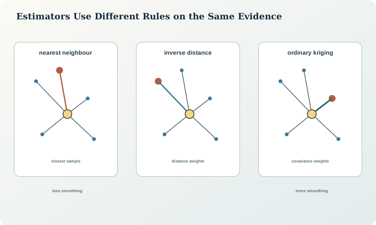
Nearest neighbour assigns the target the value of the closest eligible sample under the chosen distance metric. It preserves sample values and a data-scale distribution, so it is useful for checking global quantities and identifying the effect of smoothing. It creates abrupt boundaries and does not average to block support unless an additional support treatment is used.
Distance must respect anisotropy and domains. A closest sample across a hard boundary is not eligible merely because Euclidean distance is short.
Inverse-distance weighting
Inverse-distance weights are commonly
\lambda_i=\frac{d_i^{-p}}{\sum_j d_j^{-p}},
where p controls how rapidly influence decreases. The method is transparent and can use anisotropic distance, but it does not model redundancy among clustered samples or derive weights from the observed spatial covariance. Coincident data and very small distances require explicit handling.
Test powers and neighbourhoods. A high power approaches nearest neighbour; a low power smooths more broadly. Do not select a power only because it gives a desired grade.
Kriging framework
Kriging selects linear weights from a covariance or variogram model and the data configuration while satisfying stated mean constraints. Ordinary kriging enforces \sum_i\lambda_i=1 and treats a local unknown constant mean implicitly. Simple kriging uses a supplied mean and can be sensitive to its validity. Other forms address trends, secondary variables or non-linear targets but introduce additional assumptions.
The kriging estimate is still a conditional expectation-like smooth estimate, not a realization of local variability. Kriging variance depends on geometry, support and the covariance model; it does not directly include domain uncertainty, data errors or uncertainty in the variogram parameters.
Weight behaviour and numerical controls
Inspect weights by distance, direction and hole. Redundant data can produce endpoint dominance or negative weights. These are not automatically errors, but large cancellation can make estimates unstable and sensitive to small changes. Apply constraints only with a clear rationale and test their consequences.
Solve equations with numerical diagnostics. Near-duplicate locations, inconsistent covariance models or excessive neighbourhood size can create ill-conditioned systems. Record solver tolerances and failed estimates rather than silently substituting a value.
Method comparison and appropriate use
Run nearest-neighbour and inverse-distance checks beside the primary estimate using the same domains and comparable neighbourhoods. Compare global means, grade distributions, swaths, local differences and quantity above cut-offs. The methods are not independent votes; they reveal the effects of smoothing, continuity and weights.
An alternative method that agrees globally but differs near boundaries can expose a domain or neighbourhood issue. Disagreement in sparse areas should feed uncertainty and classification rather than be averaged away.
Synthetic worked example
At one target block, nearest neighbour gives 2.4, inverse distance squared gives 1.72 and ordinary kriging gives 1.55 units. The closest high sample shares a hole with two nearby composites, so covariance-based weights reduce their combined influence. A constrained case removes one small negative weight and changes the estimate by 0.03.
Across the domain, kriging and inverse distance have similar means, while nearest neighbour has substantially greater variance. Kriging underestimates a local high-grade swath in the synthetic known model; a shorter neighbourhood improves local response but increases estimation variance and leaves more blocks without adequate holes. Both configurations remain sensitivity cases.
Practice and review checklist
- Calculate all three methods for a small neighbourhood by hand or reproducible code.
- Plot weights by sample, hole, distance and direction.
- Compare estimates at data locations and in deliberately sparse areas.
- Quantify smoothing using variance and grade–tonnage response at equal support.
- Record numerical failures, negative weights and method-specific assumptions.
Decision record and integration
The method record should state estimator, mean assumption, variogram version, distance metric, neighbourhood, constraints, solver tolerances, support and output fields. Preserve alternative estimates with method identifiers.
Validation must compare methods consistently. Classification should not rely on a low kriging variance or close method agreement alone; both may share the same wrong domains and biased input data.
Sources
- Kriging weights in the presence of redundant data, derives linear weights and examines string effects, negative weights and comparison with inverse distance.
- Kriging with constraints, explains ordinary-kriging constraints and their optimisation basis.
- Introduction to choosing a kriging plan, connects estimator assumptions with stationarity, neighbourhood and performance.
- Mineral-resource and mineral-reserve estimation best-practice guidelines, frames method selection, documentation and comparison inside the complete resource workflow.