D3 · Publication Volume 19
Ore–Waste Boundaries
selectivity, minimum width and contact uncertainty
Learning objectives
By the end of this lesson, the learner should be able to distinguish geological, estimation, economic and operational boundaries; define a selective mining unit; apply minimum width and destination rules without double counting; represent contact uncertainty; design dig-ready boundary geometry; and evaluate misclassification consequences.
An ore–waste boundary is a decision surface, not a directly observed natural line. It combines geological continuity, estimated quality, density, a decision criterion, minimum mining width, access, equipment selectivity and timing. Several valid boundaries may therefore coexist: geological domain contact, grade envelope, design boundary and operational dig line.
Boundary hierarchy
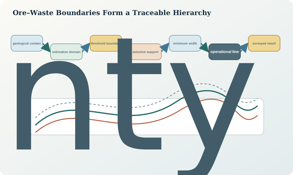
Name every boundary by type and version. A geological contact separates interpreted materials. An estimation-domain boundary controls which samples inform an estimate. A threshold boundary separates estimated classes. A design boundary incorporates minimum width and planned dilution. An operational boundary is the geometry communicated for extraction. A surveyed boundary records actual excavation.
The hierarchy must be traceable. If an operational polygon differs from the threshold contour, the transformation should identify smoothing, access, safety offsets, minimum area or equipment rules. A manual edit without a reason code breaks later diagnosis.
Selective mining unit and support
The selective mining unit is the smallest volume that can be separately classified and extracted under the stated method and conditions. Its dimensions are not simply the model cell size. They depend on equipment, geometry, control accuracy, fragmentation, visibility, access and material movement after breakage.
Evaluate grade at the selective support. A narrow high-grade interval surrounded by waste may average below the criterion when mined at practical width. Conversely, several adjacent marginal cells may form an acceptable blend parcel. The support transformation must conserve mass and contained quantity before classification.
Minimum width and edge treatment
Apply minimum width in a defined direction relative to the boundary and mining geometry. State whether internal waste is included, whether edge material is symmetrically added, and how multiple narrow bands interact. Minimum width is a design rule, not a licence to raise grade by excluding low-grade components.
For a simple ore band of true width w_o, density \rho_o and grade g_o mined with added waste width w_w, density \rho_w and grade g_w, the mixed grade per unit area is
g_m=\frac{w_o\rho_o g_o+w_w\rho_w g_w}{w_o\rho_o+w_w\rho_w}.
The same relation applies to more components after units and moisture basis are aligned.
Contact uncertainty corridor
Represent uncertainty as a corridor or alternative boundaries derived from positional error, observation spacing, geological ambiguity and model sensitivity. The corridor is not a fixed buffer unless uncertainty is actually uniform. It may widen where exposure is absent, drilling is oblique or a contact bifurcates.
Classify material inside the corridor by consequence. Options include conservative routing, isolation, additional observation, staged excavation or probabilistic assignment. Report both expected quantity and the range affected by boundary alternatives. A crisp line on a map should never imply zero positional uncertainty.
Classification errors and consequence
At a binary boundary there are four outcomes: predicted ore mined as ore, predicted waste mined as waste, waste routed as ore, and ore routed as waste. The last two are not symmetric. Their consequences depend on processing capacity, disposal, recoverability, environmental properties and opportunity cost.
Use a confusion matrix weighted by mass and contained quantity, not only cell count. Near-boundary accuracy should be assessed at selective support. Where true class is not directly observable, use a better-informed later model or bounded feed evidence with an explicit limitation.
From contour to operable geometry
Raw cell boundaries can produce jagged, narrow or disconnected polygons. Apply documented generalisation rules: minimum segment length, minimum island area, curvature or turning constraints, access offsets and topology checks. Quantify the mass and grade changed by generalisation.
Ensure the geometry uses the declared grid, elevation and vertical reference. Check closure, overlaps, gaps and orientation. Add control points that can be physically located. If the operational surface is three-dimensional, a two-dimensional line must specify the bench, level or face plane to which it applies.
Sensitivity and decision envelope
Test boundary position, threshold, minimum width, density and selectivity jointly. A one-variable sensitivity can miss interaction: widening a parcel changes both dilution and recoverability. Present a decision envelope showing which parcels retain destination under all reasonable cases, which switch, and which require more evidence.
Avoid optimising the boundary against later feed results without retaining an out-of-sample test. Retrospective tuning can explain history but may overfit. A revised rule should be tested prospectively on new parcels before broad adoption.
Synthetic worked example
A synthetic ore band is 3.2 m true width at 2.4 quality units, with adjacent waste at 0.15. The practical width is 5.0 m. After density weighting, the mixed parcel remains above the synthetic decision criterion, but a one-metre eastward contact alternative moves one end below it. The raw threshold contour also contains a 0.6 m island that cannot be separately recovered.
The released dig geometry removes the island, applies the 5.0 m width normal to the band and marks the eastern end as an isolation parcel. The release table reports the material added by width and generalisation separately. Later review can therefore distinguish planned dilution from an incorrect or unexecuted boundary.
Practice and decision record
Given a narrow synthetic lens, build the five-level boundary hierarchy. Calculate a density-weighted minimum-width grade, draw two contact alternatives, and classify parcels as stable ore, stable waste or decision-sensitive. Then generalise the line and quantify what changed.
The record should include boundary types and parents, selective unit, decision rule, minimum-width direction, density and moisture basis, uncertainty method, generalisation rules, changed quantities, coordinate reference, effective time and control points. Explain which uncertainty is geological and which comes from operability.
Sources
- Poor sampling, grade distribution and financial outcomes, connects support and sampling bias to ore–waste classification outcomes.
- Monitoring ore loss and dilution for mine-to-mill integration, discusses dilution, ore loss and boundary control across mining stages.
- Mine dilution and recovery model, provides a public technical model linking mining geometry to dilution and recovery assumptions.
- Mineral-resource and mineral-reserve estimation best-practice guidelines, covers model selectivity, geometry, support and validation considerations.