D3 · Publication Volume 19
Mine Call Factor and Root Cause
sampling, density, moisture, movement and measurement
Learning objectives
By the end of this lesson, the learner should be able to define a mine call factor on an explicit basis; decompose mass and grade components; distinguish random variation, persistent bias and timing effects; construct a causal evidence tree; test sampling, density, moisture, movement and measurement branches; control false discovery; and issue corrective actions without manipulating the balance.
A mine call factor compares called or predicted contained quantity with a later recovered or accounted quantity. Its exact numerator, denominator and direction vary in practice, so the formula must always accompany the name. A factor below or above one is a symptom. It does not identify where material changed or which measurement is correct.
Define the factor and its contract
For this tutorial, let
\mathrm{MCF}=\frac{Q_{\mathrm{accounted}}}{Q_{\mathrm{called}}}=\frac{M_a g_a}{M_c g_c},
where both contained quantities refer to the same bounded material after inventory and basis alignment. If another convention is used, label it. Report F_M=M_a/M_c and F_g=g_a/g_c beside the contained-quantity factor.
The contract names source and destination states, spatial scope, time window, dry or wet basis, sampling supports, analytical status, inventories, recoveries included or excluded, and uncertainty. Without it, two teams can publish reciprocal factors under the same label.
Establish a stable baseline
Plot period, rolling and cumulative factors with mass and grade components. Stratify by domain, extraction method, destination and measurement route. Estimate expected variation from validated historical periods or a measurement model. Control limits describe usual behaviour; they are not acceptance limits and should not be tuned to hide poor performance.
Check autocorrelation, seasonality, changing material mix and unequal period mass. A small low-mass parcel should not influence a cumulative factor like a large campaign. Weighted analysis and hierarchical grouping can distinguish a local pattern from chain-wide bias.
Causal evidence tree
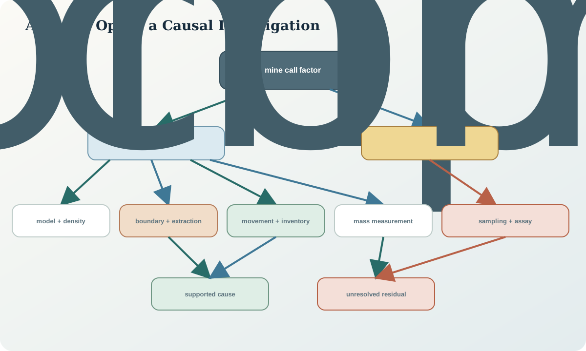
Create top branches for the called estimate, extraction, movement and inventory, accounted measurement, and comparison logic. Under the called estimate place domains, grade estimation, density, volume and moisture. Under extraction place boundary, dilution, loss and blast movement. Under accounted measurement place sampling, preparation, assay, mass measurement and process balance.
Every leaf needs a predicted signature and a test. A positive density bias raises called mass across affected domains; unrecorded stockpile growth depresses current accounted quantity and may reverse later; grade-sample contamination affects grade more than mass; coordinate displacement creates spatially coherent boundary mismatch. A cause without a distinguishing prediction is only a possibility list.
Sampling and analytical branches
Review lot definition, increment coverage, support, contamination, recovery, duplicates, blanks, reference materials, changes in method and status overrides. Compare source-specific biases on matched material where possible. A laboratory duplicate tests only part of the chain and cannot validate field representativity.
Inspect whether skewed grade distributions make a few parcels dominate contained quantity. Recalculate with validated high-value treatment and bootstrap or scenario methods where appropriate. Do not remove inconvenient values solely because the factor improves.
Density, moisture and mass branches
Trace every volume-to-mass conversion and direct mass measurement. Test density by material state and domain, including voids, swell and compaction. Align moisture conventions and sampling times. Calibrations, zero drift, belt loading, truck factors and incomplete coverage can produce mass bias.
Perform sensitivity calculations. If a plausible density correction fully explains the mass factor but not the grade factor, another branch remains. If the same density model appears in both called and accounted quantities, the apparent agreement is correlated and not independent confirmation.
Movement, inventory and time branches
Search for unmatched, duplicated, reversed or late movement events and invalid source–destination combinations. Rebuild opening and closing inventories at exact cut-off. Examine residence-time distributions and material held in broken, bin, stockpile or transport states.
Use lead–lag plots between called production and accounted feed. A correlation peak after one period supports delay, but mixing and changing grade can broaden it. Event lineage provides stronger evidence than aggregate correlation. Never shift periods selectively until a favourable factor appears.
Statistical testing and uncertainty
Separate measurement uncertainty from process variation and model uncertainty. Use paired differences when the same parcels are observed at two stages. Examine confidence intervals and practical consequence, not only a significance threshold. Multiple domains, periods and attributes create many opportunities for chance findings; predefine primary tests and seek replication.
When propagating uncertainty, include covariance and shared inputs. A factor distribution may be asymmetric, especially when the denominator is uncertain. Scenario or resampling methods can be clearer than a symmetric error bar. Report the unresolved portion honestly.
Corrective action and verification
Actions should target verified or high-priority causal controls: repair an identifier workflow, change a sampling increment, calibrate a mass measure, revise a density domain, add a survey, isolate uncertain material or update a model rule. Each action needs an expected signature, owner function, effective date and verification dataset.
Do not “correct” historical source measurements merely to align the factor. A justified calibration correction preserves raw and corrected values. Prospective verification on later material is stronger than reusing the discovery period. Close an action only when the predicted signature improves without creating a new imbalance elsewhere.
Synthetic worked example and investigation record
The synthetic contained-quantity factor is 0.91 for three periods. Mass factor is 0.98 and grade factor is 0.93. The pattern is concentrated in wet control holes and disappears in dry-hole parcels; a stockpile timing correction changes mass but not grade. Pulp duplicates are stable, while field duplicates from wet holes show a negative shift and high dispersion.
The evidence supports a field collection and splitting branch, not a general analytical correction. A revised capture protocol is tested prospectively on the next parcels, with dry holes retained as a comparison group. Build the causal tree, quantify how much each supported correction changes the factor, and keep the remaining residual unresolved until independent evidence arrives.
Sources
- Reconciliation along the mining value chain, discusses mine call factors, variability, measuring points and cause-and-effect investigation.
- Monitoring ore loss and dilution for mine-to-mill integration, links timing, movement, dilution and ore loss to mine-to-feed factors.
- Poor sampling, grade distribution and financial outcomes, analyses the effects of sampling error and bias across different grade distributions.
- Combined standard uncertainty, explains combining uncertainty components and recognising systematic effects.