D5 · Publication Volume 21
Deleterious Elements and Product Quality
penalties, blending and constraints
Learning objectives
By the end of this lesson, the learner should be able to distinguish elemental concentration from mineral host and product consequence; translate a product specification into measurable constraints; calculate contained impurity and simple blending limits; recognise threshold, penalty and rejection logic; trace impurities through products, residues and solutions; assess variability at the relevant delivery support; and construct a product-quality ledger without presenting hypothetical commercial terms as current facts.
Define quality at the receiving boundary
Product quality is the set of chemical, mineralogical and physical properties used to determine whether a material is fit for its downstream destination. It can include valuable-component grade, deleterious elements, moisture, particle size, mineral form, radioactivity, handling behaviour and variability. Requirements are product-, destination-, contract- and time-specific. This tutorial uses synthetic limits only.
Translate each requirement into analyte, method, sample support, moisture basis, unit, averaging period, threshold type and consequence. Distinguish target, guaranteed minimum, penalty band, rejection limit and informational property. A laboratory concentrate does not become saleable because its target grade is high; every controlling property and downstream route needs evidence.
Host minerals and deportment
An element may occur in the target mineral lattice, a separate impurity mineral, gangue inclusions, surface coatings or process water. Host determines removability. Grinding can liberate a discrete impurity; flotation chemistry can separate surfaces; leaching may dissolve target and impurity together; a lattice-bound element may persist through concentration. Bulk assay cannot identify which mechanism is available.
Create an impurity-deportment table by feed domain, size, mineral host and stream. Include the unassigned fraction and analytical limitations. Track whether a change in total concentration arises from real mineralogical variability, recovery of a host, dilution by another stream or moisture. When host evidence is weak, preserve competing hypotheses and test them.
Product and residue mass balance
For component j, contained mass in a stream is C_j=M g_j. Across a process boundary,
$\sum C_{j,\mathrm{in}}+C_{j,\mathrm{generation}}=\sum C_{j,\mathrm{out}}+\Delta I_j,$
where generation is normally zero for an element but chemical forms can change, and \Delta I_j is inventory change. An impurity removed from product has not disappeared; it reports to tailings, residue, solution, gas, bleed or inventory. Characterise that destination and its consequence.
Use dry basis consistently and include moisture when contracts or transport depend on it. A low impurity concentration in a large residue can contain most of the impurity. Conversely, a small product stream can be enriched above a limit. Report recovery or deportment of the impurity together with concentration.
Blending and threshold logic
For two dry streams A and B with impurity grades g_A and g_B, a simple blend grade is
$g_{\mathrm{blend}}=xg_A+(1-x)g_B,$
where x is the dry-mass fraction of A. If a maximum grade g_{\max} lies between the two, the algebraic limit can be solved for x. This calculation assumes representative grades, additive contained mass, no process interaction and the same basis.
Real blending must consider uncertainty, parcel size, segregation, time windows and correlated valuable grade. An average below a limit can conceal individual parcels above rejection. The safe operating target may require a buffer supported by measurement and consequence analysis. Do not invent a universal buffer or assume that dilution is always an acceptable control.
Penalties, payability and net product value
A synthetic net product value can be represented as gross payable value minus treatment, refining, transport, moisture and impurity adjustments. Each term must state unit and basis. Penalty schedules are often piecewise: no adjustment below a threshold, increasing charges within bands and rejection beyond a limit. A smooth average cannot reproduce a discontinuity.
Date and source every commercial assumption in real work. Use ranges and alternative destinations where evidence supports them. Product value can change without geology changing, and a new impurity limit can change domains or cut-off. The curriculum teaches the structure, not a price forecast, contract or investment recommendation.
Sampling and short-term variability
Product sampling must represent the lot or delivery period. Fine particles segregate, moisture varies, and rare impurity minerals can be heterogeneously distributed. Define lot, increment selection, sample preparation, analytical method and uncertainty. Compare the support of testwork composites, block predictions, daily production and shipment specifications.
Short-term excursions matter when the receiving boundary evaluates parcels rather than annual means. Simulate or test sequences, stockpile mixing and measurement delay. A block model with smooth estimates may understate local variance. Product-quality control needs leading indicators and confirmatory measurements with response rules.
Process controls and trade-offs
Controls can include selective mining, stockpiling, blending, grind changes, reagent conditions, separation stages, impurity removal, solution purification and alternative product routing. Each has capacity, delay, loss and cost. Increasing selectivity may reduce target recovery; impurity rejection may transfer environmental burden; extra cleaning can lower mass yield and throughput.
Use a constraint table with measured state, predicted state, uncertainty, control range, response time and consequence. Do not treat blending as a remedy for unknown measurements. When no credible control keeps product within specification, the pathway must be revised or held.
Uncertainty and common failure modes
Failure modes include treating a bulk element as one mineral, using a quoted specification without version or destination, mixing dry and wet basis, averaging across a rejection threshold, ignoring analytical reporting limits, omitting impurity destinations, and optimising target recovery alone. Another is assuming that a product term remains valid throughout a project or across markets.
Quantify assay uncertainty, sampling variance, spatial prediction error, process-response error and commercial scenario uncertainty separately. Explore correlation between target and impurity. A high-grade domain can also carry more penalty mineral. Report probabilities or scenarios at the parcel support rather than claiming certainty from smoothed block estimates.
Interfaces and transferable data
The quality ledger links requirement versions, analytes, hosts, domains, test products, process streams, parcels, measurements, predicted distributions and destinations. Geological models store mineral or elemental attributes with uncertainty. Process models predict deportment. Commercial models apply dated terms. No one layer should hard-code the others invisibly.
When a specification changes, identify affected tests, products, blocks and decisions through version links. Preserve whether a limit is confirmed, indicative or synthetic. Source organisations and counterparties, if any, belong in controlled source or contract records, not in general instructional prose.
Integration checkpoint
Reconcile target and impurity masses, test the parcel support against the specification period, and propagate the current requirement version through blend, process, residue and value models. The quality decision remains conditional wherever host, measurement or commercial evidence is incomplete.
Synthetic worked example
Synthetic concentrate A has 0.42% impurity Z and concentrate B has 0.08% Z. A provisional teaching limit is 0.20%. Solving 0.20=x(0.42)+(1-x)(0.08) gives x\approx0.353, so the deterministic blend can contain at most about 35.3% A. However, assay and parcel variability make 35.3% an equality with no protection against exceedance.
The decision record evaluates lower A fractions under uncertainty, target-component grade, available B inventory and product timing. Mineralogy shows Z occurs partly in a separately floating phase, so a cleaner test is also scheduled. Rejecting that phase changes tailings chemistry and is included in the boundary. All grades, limits and terms are synthetic.
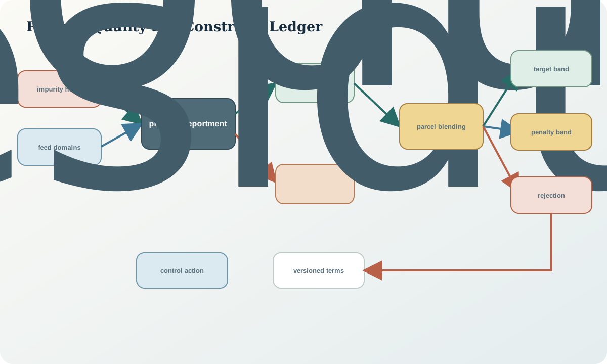
Conceptual figure
Practice and decision record
Create two synthetic concentrates with target and impurity grades. Calculate a deterministic blend limit, then add uncertainty and a parcel-based rejection condition. Trace the impurity to every output and propose one geological and one processing control. Write a quality record with specification version, basis, sampling support, host evidence, scenarios, controls and escalation trigger.
The record fails if it presents synthetic terms as current, averages across rejection without parcel analysis, loses the impurity outside product, or claims a mineral host from elemental assay alone.
Sources
- Practice Guidelines for Mineral Processing, 2022, guidance on contaminants, saleable products, off-site treatment, sampling and cost assumptions.
- Australasian Code for Reporting of Exploration Results, Mineral Resources and Ore Reserves, 2012, source example for material product, metallurgical and market assumptions.
- Critical minerals in magmatic-hydrothermal systems, public synthesis illustrating mineral hosts, processing routes, impurities and accounting boundaries.