D4 · Publication Volume 20
Hydrogeology Foundations
aquifers, hydraulic head, flow, dewatering and water quality
Learning objectives
By the end of this lesson, the learner should be able to build a mine-interface hydrogeological conceptual model; calculate hydraulic head, gradient, specific discharge and simple water balance; distinguish conductivity, transmissivity and storage; recognise fractured-flow and boundary uncertainty; design basic monitoring and testing logic; and connect inflow, depressurisation, dewatering and water quality to mine decisions.
Water occurrence and conceptual model
Groundwater occupies connected pores and fractures below or within variably saturated ground. Aquifers transmit useful quantities of water; aquitards transmit more slowly at the relevant scale; boundaries may be hydraulic, geological or operational. These labels are scale- and purpose-dependent. A fractured unit can transmit little through its matrix yet carry large flow along sparse structures.
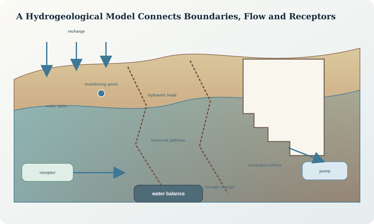
Begin with a three-dimensional conceptual model: topography, weathering, units, structures, recharge, discharge, surface water, pressure compartments, existing excavations, wells, sumps and receptors. State model limits and time period. Include alternative connectivity scenarios where evidence is sparse.
Hydraulic head and gradient
Hydraulic head combines elevation and pressure potential. For water of density \rho, h=z+p/(\rho g). Compare heads only when elevation datum, density assumption, screened interval and measurement time are compatible. Water depth below collar is not head until collar elevation and reference are applied.
Hydraulic gradient is change in head over distance in a stated direction, i=\Delta h/\Delta l. Use screened positions, not just collar separation. A map gradient can miss strong vertical flow. Measurement uncertainty becomes important when head differences are small relative to survey or sensor error.
Darcy flow and hydraulic properties
For a saturated porous-medium idealisation, specific discharge is \mathbf{q}=-\mathbf{K}\nabla h. Volumetric flow through area A in a one-dimensional isotropic case is Q=-KA\Delta h/\Delta l. The negative sign indicates flow down head gradient. Average pore-water velocity also depends on effective porosity.
Hydraulic conductivity K describes the medium-fluid capacity to transmit water. Transmissivity integrates conductivity through saturated thickness, often T=Kb for a uniform layer. Storage describes water released or taken up per head change. These properties span orders of magnitude; geometric means, ranges and spatial domains are often more informative than arithmetic averages.
Fractured and heterogeneous flow
Fracture flow depends on aperture, roughness, infill, connectivity, stress and scale. A high-conductivity test interval does not prove regional connectivity, while a low test can miss a transmissive feature. Faults may be conduits, barriers or both along different segments. Weathered zones and contacts can redirect flow.
Use multiple evidence types: core and imagery, hydraulic tests, head response, chemistry, temperature, tracers where appropriate, excavation inflow and structural mapping. Treat connectivity as a hypothesis to test. Numerical grids must preserve important pathways or represent their effect through defensible upscaling.
Recharge, boundaries and water balance
Recharge may arise from rainfall, losing streams, storage facilities, irrigation or operational water. Boundaries include rivers, drains, no-flow divides, specified heads, fluxes and moving excavation faces. Their position and behaviour can change through seasons and mining.
A control-volume balance is
$\Delta S = I_{\text{recharge}}+I_{\text{boundary}}+I_{\text{operations}}-Q_{\text{pumping}}-Q_{\text{discharge}}.$
Define sign, period, moisture and density basis. Balance closure does not identify every pathway; residual may combine measurement error, storage and omitted flow.
Inflow, depressurisation and dewatering
Mine inflow is water entering an excavation. Dewatering removes water to maintain workable conditions or intercept flow; depressurisation lowers pore pressure for stability. A sump pump can control nuisance water without depressurising a slope, while pressure wells can improve stability with modest discharge. Keep objectives and performance metrics separate.
Design questions include expected and credible peak inflow, storage, redundancy, power, discharge route, treatment, drawdown extent, subsidence or receptor effect and recovery after outage. Probe drilling and cover drilling may provide advance warning underground. This tutorial supplies no pumping design or discharge approval.
Monitoring and hydraulic testing
Monitoring locations follow the conceptual model and decision. Record collar, screened interval, construction, datum, sensor, calibration, barometric or density corrections, sampling interval and access. Nested points can reveal vertical gradients. Manual checks provide independent control for automated records.
Tests include slug, packer, pumping, recovery and interference methods, each with geometry and assumptions. Analyse diagnostic plots and alternative models; do not accept a software fit without checking boundary effects, wellbore storage and heterogeneity. Preserve raw pressure, rate and time data.
Water quality and material interaction
Water quality affects handling, treatment, corrosion, environment and interpretation. Field parameters, major ions, trace components and suspended solids require suitable sampling, preservation, quality control and chain of custody. Chemistry can help identify mixing but rarely proves a unique source.
Excavation exposes reactive minerals and changes oxygen, flow and contact time. Separate geochemical source, transport pathway and receptor. Link predictions to mineralogical evidence and water balance. Do not extrapolate one sample across a changing system.
Model calibration, prediction and uncertainty
Calibrate to multiple states where possible: heads, inflows, drawdown, recovery and seasonal response. Calibration is not validation and non-unique parameter sets can fit the observations. Use sensitivity, scenarios and predictive intervals. Reserve data for independent checks when feasible.
Record predictions as ranges conditional on boundary, property and mining scenarios. Define monitoring that tests the load-bearing assumptions. Update when excavation reveals new structures or response diverges, preserving prior forecasts for learning.
Synthetic worked example
Three synthetic piezometers have heads of 612.4, 607.1 and 603.8 m in the same datum. The first and second screens are 180 m apart along a fractured corridor, giving a simple gradient magnitude of about 0.029. A test suggests K between 2\times10^{-7} and 3\times10^{-6}\,\mathrm{m/s}, a range too wide for a single deterministic inflow forecast.
The planned excavation intersects the corridor between the second and third points. The review carries low-, central- and high-connectivity scenarios, adds an observation point across the structure, reserves storage and pump redundancy for the high case, and defines a pressure response that triggers geotechnical review. It does not infer regional drawdown from the three points.
Practice and hydrogeological record
Calculate head and gradient for a three-point synthetic section, then compute a Darcy-flow range using two conductivities. State every assumption and why the calculation is not a pump design. Create a conceptual-model record with domains, boundaries, stresses, observations, tests, water balance, uncertainty scenarios, receptors, control objectives and update triggers.
A passing record preserves datum and screen identity, separates inflow control from depressurisation, and makes no claim of zero connectivity merely because a test is dry.
Sources
- Introduction to ground-water hydraulics, United States Geological Survey.
- General facts and concepts about ground water, United States Geological Survey.
- Theory of aquifer tests, United States Geological Survey.
- Groundwater susceptibility and Darcy-flow concepts, United States Geological Survey.