C5 · Publication Volume 15
Mineral Spectroscopy
absorption features, continuum removal and mixtures
Learning goals
This lesson develops reflectance spectroscopy as a measurement of material–energy interaction rather than a fingerprint lookup. The learner should be able to connect absorption mechanisms to feature regions; estimate continuum and feature metrics; explain grain size, abundance and mixture effects; reconcile library, field and image spectra; design calibration and quality control; and state the level of mineral inference supported by the evidence.
A spectral match is conditional on wavelength calibration, response, geometry, material state and scale. Similar curves can arise from mixtures or different mechanisms, and the absence of a feature may reflect masking, low abundance, unsuitable grain size, atmosphere or sensor resolution.
Absorption mechanisms and diagnostic regions
Electronic transitions and charge-transfer processes can produce features in visible and near-infrared wavelengths, including responses associated with iron-bearing materials. Vibrational overtones and combinations produce many short-wave infrared absorptions associated with bonds involving hydroxyl, water, carbonate and other molecular groups. Fundamental vibrations and lattice behaviour contribute in thermal infrared regions.
A mineral group may share a feature region while composition, crystallinity or chemical substitution shifts position and shape. Conversely, one mineral can show several features with different sensitivities. Identification should use a coherent set of features, continuum and known sensor response rather than one minimum.
Atmospheric gases also absorb at specific wavelengths. Detector joins, low-signal intervals, stray light and residual atmospheric correction can imitate or distort material features. Mark unusable wavelength intervals before searching for absorptions.
Continuum, feature position, depth and shape
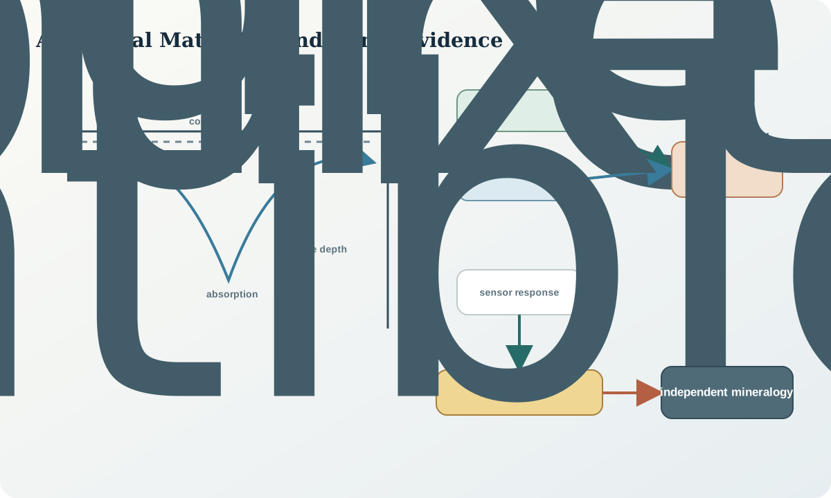
A continuum is an estimated background envelope across an absorption. Continuum removal divides the spectrum by that envelope so feature shape can be compared separately from broad brightness and slope. The result depends on anchor selection and continuum model. Anchors inside neighbouring features or noisy intervals bias depth and centre.
For continuum-removed reflectance R_c(\lambda), band depth may be described as D=1-R_c(\lambda_m) at a selected minimum \lambda_m. Feature area integrates 1-R_c across declared bounds. Centre can be the sampled minimum, a local polynomial estimate or a model parameter; each has different sensitivity to sampling and noise.
Report bounds, continuum, smoothing, interpolation and uncertainty. Do not quote a feature centre more precisely than spectral calibration and response support. Compare the full residual and alternative fits, not only the best-match score.
Grain size, surface state and mixtures
Reflectance depends on grain size, packing, roughness, coatings, porosity, moisture and illumination. Increasing optical path length can deepen absorptions until saturation while lowering overall reflectance, but behaviour varies with material and mixture. Weathered rinds or coatings may dominate a remote surface even when the underlying rock differs.
An areal mixture combines subpixel surface fractions and can often be approximated linearly in reflectance under common illumination. An intimate mixture allows photons to interact with several constituents and is generally nonlinear. Shadows add a low-energy component; vegetation, water and soil organics introduce their own features. Low abundance can be detectable for a strong feature yet unquantifiable without an appropriate radiative model.
Treat abundance estimates as model-dependent. A high match score does not imply purity, and a feature-depth map is not automatically a concentration map. Use controlled mixtures and independent mineralogy when quantitative claims matter.
Spectral libraries and transfer across scales
A useful library record includes sample description, preparation, grain size, measurement geometry, illumination, reference standard, instrument, wavelength calibration, spectral resolution, quality flags and independent composition. A curve without this context is not a transferable reference.
Before comparing to imagery, convert compatible physical quantities, remove invalid wavelengths and convolve high-resolution spectra to the image sensor response. Apply the same continuum or normalisation to reference and observation. Library spectra measured on pure powders may not represent weathered, mixed or vegetated field surfaces.
Build a candidate set that includes likely materials, confounders and mixtures. Evaluate whether candidates remain separable after convolution and realistic noise. If two candidates collapse to the same response, report a group or feature class rather than choosing the highest numerical score.
Field and laboratory measurement quality
Field spectroscopy requires stable illumination or a characterised source, a traceable reflectance reference, appropriate foreoptic, known field of view, dark-current and white-reference checks, and geometry records. Reference frequency should respond to illumination change. Shadows cast by the operator or instrument, variable clouds and mixed support can dominate subtle geology.
Laboratory measurements improve control but introduce preparation choices. Record whether the sample is intact, crushed, sieved, dried or heated, and preserve representative material for independent mineralogy. Repeat orientations for anisotropic or rough samples and repeat preparation where heterogeneity matters.
Quality control includes wavelength and radiometric checks, repeat spectra, reference materials, bad-channel masks and drift monitoring. Link every spectrum to a sample or field support and every derived feature to the raw scan. Rejecting a spectrum requires a recorded criterion and retained original.
Worked synthetic example
Three synthetic candidates have absorptions near 2.20\,\mu\mathrm m. Candidate A has a symmetric feature at 2.205\,\mu\mathrm m plus a weaker feature at another diagnostic interval. Candidate B has an asymmetric minimum at 2.215\,\mu\mathrm m. Candidate C is a mixture whose broad depression spans both. At laboratory resolution all differ. After convolution to broad image bands, A and B become indistinguishable and C differs mainly in depth.
An image pixel matches A slightly better than B, but spectral calibration uncertainty is larger than their convolved difference and the secondary feature is not sampled. The correct inference is a compatible mineral group, not Candidate A. A field spectrum with finer response plus independent mineralogy is the discriminating test.
Interpretation and decision. Report feature existence, position interval, depth, shape, quality and compatible candidates separately. Explain how mixture, grain size, moisture and sensor response affect the claim. Use “spectrally consistent with” when identity is not independently confirmed, and map unknown where signal or exposure is inadequate.
Practice and audit checklist
Create synthetic spectra for two pure candidates and three mixtures. Add continuum slope, wavelength shift and correlated noise; then convolve them to two sensor responses. Compare raw, continuum-removed and derivative representations. State which identifications survive and design the minimum field/laboratory validation set.
Audit questions: Are wavelength and reflectance units explicit? Were atmospheric and bad channels removed? Is the continuum documented? Were references convolved to response? Are grain size and geometry compatible? Does score uncertainty separate the leading candidates? Is an abundance claim supported by a mixing model and independent measurement?
Sources
- USGS Spectral Library, provides spectra with material descriptions and independent analytical context.
- Spectral Library Version 7 report, documents measurement, sample and library structure for minerals, rocks, soils, mixtures and other materials.
- High-resolution spectral library overview, explains wavelength resolution, mixtures and remote material detection.
- Continuum and baseline processing methods, documents baseline removal and other reproducible spectral-analysis operations.