C5 · Publication Volume 15
DEMs, LiDAR and Terrain Products
elevation, slope, aspect, hillshade and artefacts
Learning goals
This lesson treats topography as a measured surface with scale, datum, classification and uncertainty. The learner should be able to distinguish point cloud, surface model and bare-earth model; audit horizontal and vertical references; compute and interpret slope, aspect and hillshade; recognise interpolation, striping and hydrologic artefacts; choose analysis scale; and integrate terrain evidence without turning shaded relief into a unique geological structure.
Terrain can reveal landforms, drainage, scarps, lineaments and surface processes, but elevation is not bedrock geology. Vegetation, buildings, water, interpolation and filtering influence the surface. Derivatives amplify both morphology and error.
Point clouds, surface models and bare earth
Laser ranging estimates distance from pulse travel time combined with platform trajectory, attitude, scan geometry and calibration. A pulse can yield one or several returns from canopy, structures and ground. Point classification assigns ground, vegetation, building, water, noise or other categories; classification error transfers into derived surfaces.
A digital surface model represents an upper reflective surface and may include vegetation or structures. A digital terrain or bare-earth model estimates the ground surface after classification and interpolation. A generic digital elevation model can refer to either unless metadata states the surface. Photogrammetric elevation derives from image correspondence and has different failure modes from lidar.
Point density, pulse spacing, scan angle and overlap affect sampling, but nominal density alone does not define accuracy or resolvable landform. Inspect spatial density, flight-line overlap and classification by terrain and cover.
Horizontal, vertical and temporal reference
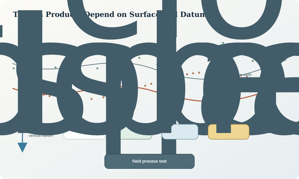
Elevation requires a horizontal coordinate reference, horizontal datum, vertical datum, height type and units. Ellipsoidal height and orthometric height differ by a geoid model. Combining surfaces with different datums can create regional offsets or tilts that resemble uplift, erosion or drainage change.
Trajectory and control error can create strip offsets, boresight patterns and local warps. Report checkpoints independent of calibration and stratify vertical error by land cover and slope. Root-mean-square error alone does not describe bias or heavy tails.
Acquisition date matters because vegetation, water, snow, construction and surface disturbance change. A mosaic may combine projects, sensors, datums and seasons. Maintain a source index per cell or tile and avoid interpreting seam boundaries as terrain.
Gridding, interpolation and scale
Point-to-raster interpolation selects a cell size, statistic, neighbourhood, breakline treatment and empty-cell rule. A very small cell relative to point spacing produces holes and unstable facets; a large cell smooths scarps and channels. Triangulated surfaces preserve points but can bridge gaps. Hydrologic breaklines and flattening modify water surfaces for a stated purpose.
Resampling a DEM changes derivative behaviour. Downsampling should consider terrain roughness and whether mean, minimum, maximum or another statistic matches the question. Smoothing reduces noise and small morphology together. Record filter scale and compare results at multiple supports.
Resolution should match the landform. A fault scarp, broad ridge and catchment divide require different neighbourhoods. Map the effective support of the derivative, not only output pixel size.
Slope, aspect, curvature and hillshade
Slope and aspect derive from local elevation gradients. With horizontal derivatives p=\partial z/\partial x and q=\partial z/\partial y, slope angle is \theta=\arctan\sqrt{p^2+q^2}. Aspect needs an explicit compass convention and is undefined on flat surfaces. Derivative kernels and cell size affect both.
Curvature measures changes in gradient and can highlight ridges, valleys or breaks of slope, but second derivatives strongly amplify elevation noise. State whether profile, plan, mean or another curvature is used and its units or scaling.
Hillshade simulates illumination from selected azimuth and altitude. It is a visual derivative, not measured reflectance. A lineament parallel to illumination may disappear; a seam or noise band may be enhanced. Use several illumination directions or multidirectional shading and confirm features in elevation profiles, slope and source points.
Artefacts, drainage and geological inference
Common artefacts include flight-line striping, scan-edge error, interpolation triangles, vegetation remnants, building pits, water-edge steps, tile seams, void fills and quantised contours. Hydrologic conditioning can breach, fill or flatten terrain, altering natural depressions and channel gradients. Inspect provenance before geomorphic interpretation.
A lineament is an aligned surface expression, not automatically a fault. It may follow lithological contrast, joints, drainage engineering, track, vegetation edge, illumination or artefact. A scarp may be tectonic, erosional, depositional or human-made. Test continuity across products and use cross profiles, drainage relations, surface age and field evidence.
Terrain evidence is strongest when it makes different predictions under competing process hypotheses. For example, an active displacement hypothesis may predict consistent offset markers and scarp degradation; an erosional boundary may follow drainage and substrate contrasts without displaced markers.
Worked synthetic example
A synthetic bare-earth grid shows a 1.2 m step across a low-relief plain. A single northwest hillshade displays a striking linear scarp. Source-point inspection reveals that half the feature coincides with a flight-line boundary and a 0.5 m vertical strip offset; the other half persists across overlaps and in independent profiles. After strip adjustment, the artefactual half disappears while a shorter curved break remains.
The remaining feature is compatible with either an erosional terrace edge or displacement. Drainage truncation and field sediment relationships are the discriminating evidence. The output maps verified morphology, artefact-affected support and two process hypotheses rather than a continuous fault trace.
Interpretation and decision. State the measured terrain feature, its height, length, orientation, support and uncertainty before assigning origin. Show sensitivity to illumination and derivative scale. A field-check route should cross the feature, artefact boundary, apparent continuation and negative control.
Practice and audit checklist
Generate a synthetic point cloud containing a scarp, channel, building, canopy and strip offset. Classify and grid it at two cell sizes; compute slope, aspect and four hillshades. Compare the source points and derivatives, map artefacts and write two process explanations. Specify the field observations needed to decide between them.
Audit questions: Is the surface DSM or bare earth? Are horizontal and vertical datums explicit? Is source density adequate? Were classification and breaklines reviewed? Are derivative kernel and units recorded? Does the feature persist across illumination and support? Are seam and acquisition dates mapped? Is geological origin independently tested?
Sources
- 3D elevation products and services, distinguishes point clouds, elevation models and terrain derivatives.
- Elevation standards and specifications, documents quality levels, metadata, accuracy and deliverable requirements.
- Spatial metadata for elevation sources, explains work-unit provenance and validated source availability.
- Elevation-derived hydrography source requirements, documents datum, resampling, breakline and source controls for terrain-derived products.