C5 · Publication Volume 15
Change Detection and Time Series
registration, seasonality, disturbance and monitoring
Learning goals
This lesson makes change a hypothesis about a time-indexed measurement process. The learner should be able to define change object and baseline; harmonise geometry, spectral response and processing; screen clouds, shadow and missing observations; separate trend, seasonality and abrupt break; estimate change uncertainty; prevent multiple-comparison and training leakage; and report persistence, confidence and attribution limits.
A difference image is not automatically change. It contains real surface variation plus illumination, atmosphere, view angle, sensor, calibration, registration, resampling and mask differences. Attribution needs a causal model and independent evidence.
Define the change object and baseline
Specify whether the target is spectral magnitude, class, boundary, elevation, morphology, temperature, disturbance footprint or another property. State minimum size, duration and consequence. A transient observation and persistent state change require different rules.
Choose a baseline that represents expected variability, not merely one convenient date. Use multiple observations when seasonality and noise matter. A historical median, seasonal model or pre-event distribution can be more robust than a single reference image. Record gaps and changes in product generation.
Predefine the analysis unit and date rule. Pixel-level, object-level and landscape-level changes have different uncertainty and multiple-testing burdens. If the target date is selected after inspecting the largest difference, validation must account for that selection.
Harmonisation and masks across time
All observations need compatible physical quantities, response functions, spatial grids, datums and processing. Cross-sensor time series may require bandpass adjustment, common atmospheric correction, bidirectional normalisation and co-registration. These operations reduce but do not eliminate differences.
Build a per-date validity mask for cloud, shadow, snow, saturation, aerosol, low illumination and other product flags. Cloud-edge and shadow contamination often require conservative dilation. A temporal composite must retain which date contributed to each pixel; otherwise apparent boundaries can be acquisition seams.
Do not fill long gaps silently. Interpolation creates modelled values and smooths abrupt events. Preserve observed, modelled and missing status. Report usable observation density and its spatial pattern.
Differencing, indices and object change
Direct difference \Delta x=x_{t_2}-x_{t_1} is interpretable when quantities and support are compatible. Relative change becomes unstable near zero. Normalised indices can reduce common brightness but inherit ratio limitations. Change-vector analysis combines several bands and requires covariance and scaling.
Post-classification comparison summarises class transitions but compounds errors from both maps. An apparent rare transition can be dominated by classification confusion. Propagate confusion or validate transitions directly. Object-based methods can enforce minimum size and shape, but segmentation parameters become part of the change definition.
Thresholds should follow expected error and consequence. Map continuous change magnitude and uncertainty along with a decision class. Evaluate stable controls and inject synthetic changes to estimate sensitivity.
Trend, seasonality, breaks and persistence
A time series can be represented as y_t=T_t+S_t+\epsilon_t, with trend T_t, seasonal component S_t and residual \epsilon_t. Abrupt-change models add one or more breaks. Components are not uniquely determined when sampling is sparse or the record is short. Harmonic models assume recurring structure that may itself change.
Seasonality can mimic geology-related change through vegetation, moisture, snow or solar geometry. Compare like seasons or model season with adequate years and observations. Persistence rules reduce one-date false alarms but delay detection and can miss brief real events.
Autocorrelation reduces independent information. Use time-aware validation: do not randomly split neighbouring dates from one event into train and test. Test performance before, during and after known synthetic events and across quiet periods.
Uncertainty, attribution and multiple testing
For independent dates, variance of a difference is \sigma_{\Delta}^2=\sigma_1^2+\sigma_2^2; shared calibration or atmosphere adds covariance terms. Registration error creates value uncertainty proportional to local gradient. Estimate change significance with these spatially varying terms rather than one universal threshold.
Testing millions of pixels makes some extreme values inevitable. Control false discoveries, require spatial or temporal coherence, or define objects before testing. Do not tune threshold and then quote validation from the same anomalies.
Detection answers whether a measured state changed. Attribution asks why. Fire, rainfall, vegetation management, excavation, sensor processing and natural geomorphic processes can share signatures. Use external records, multi-sensor evidence and field checks. Report compatible causes and the observation that would distinguish them.
Worked synthetic example
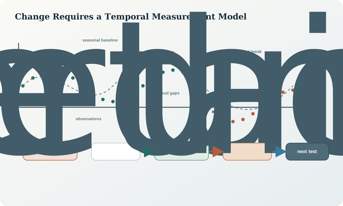
A synthetic five-year monthly reflectance series has a stable seasonal cycle, irregular cloudy gaps and one persistent 8% decrease beginning in year four over a small area. A two-date comparison against a wet baseline exaggerates the decrease across the whole scene. A seasonal harmonic model reduces the regional effect, but registration error produces false edges along a road.
After local co-registration uncertainty is included and road edges are excluded, the small area shows a persistent residual for eight valid observations. The change is detected. Cause remains ambiguous between surface disturbance and vegetation loss because both predict the observed bands. A terrain change measure and field observation are the next discriminating tests.
Interpretation and decision. Report magnitude, onset interval, duration, valid observations, baseline, uncertainty and excluded support. Use “persistent spectral change” rather than assigning a cause without evidence. The decision rule must state how future observations confirm, reverse or retire the alert.
Practice and audit checklist
Generate a synthetic seasonal time series with clouds, sensor transition, subpixel shift, transient moisture pulse and persistent disturbance. Compare two-date, seasonal-model and object-based detection. Use stable controls and time-blocked validation. Produce change magnitude, uncertainty, persistence, cause alternatives and next-test maps.
Audit questions: Is baseline representative? Are products harmonised? Is per-date validity retained? Are missing values distinguished from filled values? Is registration uncertainty gradient-aware? Was seasonality modelled with adequate support? Are threshold and validation independent? Is detection separated from attribution?
Sources
- Analysis-ready time-series product contents, documents common grids, surface products, quality masks and metadata for repeat analysis.
- Harmonized Landsat and Sentinel-2 user guide, specifies cross-sensor atmosphere, geometry, bandpass and bidirectional harmonisation.
- Land-change time-series science products, documents harmonic modelling of seasonality, trend and breaks from quality-screened observations.
- Level-1 time-series geometry criteria, explains why geometric quality tiers matter for repeat observation.