B3 · Publication Volume 8
Deforming Grids and the Strain Ellipse
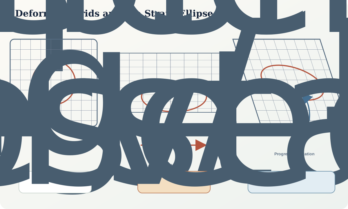
pure shear, simple shear, rotation and finite strain
Learning objectives
After this lesson, you should be able to map points with a deformation gradient; distinguish translation, rigid rotation and strain; compare pure shear with simple shear; derive principal stretches from a finite-strain tensor; explain the strain ellipse and ellipsoid; and state why a final shape does not uniquely preserve the deformation path.
Start with a field problem
An originally near-circular pebble population is now elliptical. Long axes define a foliation and small tails appear rotated relative to the matrix. Did the rock undergo coaxial flattening, simple shear, multiple increments with changing axes, rigid rotation of anisotropic pebbles, pressure solution, or selective survival of particular clasts?
The final ellipse provides a finite-state constraint, not an automatic movie. Different sequences of pure shear, simple shear and rotation can yield similar axial ratios and orientations. The original objects may not have been circular, may have behaved more rigidly than the matrix or may have changed volume. A deformed grid is useful because it makes the assumed starting geometry and coordinate transformation explicit.
Core process model
For a locally homogeneous deformation, a material vector in the reference state, d\mathbf{X}, maps to the current state as
d\mathbf{x}=\mathbf{F}\,d\mathbf{X},
where \mathbf{F} is the deformation gradient. Its determinant J=\det\mathbf{F} is the local volume ratio. The right Cauchy–Green tensor \mathbf{C}=\mathbf{F}^{T}\mathbf{F} removes rigid-body rotation and describes stretch relative to the reference coordinates. The square roots of its eigenvalues are principal stretches.
Plane pure shear can be represented by
\mathbf{F}_{p}=
\begin{bmatrix}
\lambda & 0\\
0 & 1/\lambda
\end{bmatrix},
for an area-preserving case. Principal directions remain fixed and material lines do not experience bulk rigid rotation, although their orientations change as axes stretch unequally. Plane simple shear can be represented by
\mathbf{F}_{s}=
\begin{bmatrix}
1 & \gamma\\
0 & 1
\end{bmatrix},
where \gamma is engineering shear. Simple shear is non-coaxial: material lines and the instantaneous stretching directions rotate through the deformation.
A unit circle maps to a strain ellipse. In three dimensions a sphere maps to an ellipsoid with stretches X\geq Y\geq Z. Shape may be described by ratios such as X/Y and Y/Z, but an ellipsoid does not by itself reveal vorticity, sequence or time. The same finite ellipsoid can arise from different paths because matrix multiplication is order dependent and because the rotational part may differ.
Natural deformation is commonly heterogeneous. \mathbf{F} varies in space, and strain gradients bend lines and distort formerly parallel surfaces. A strain ellipse at one point should not be silently extended across a fold hinge, shear-zone boundary or lithological contrast.
Evidence and measurement
Useful strain markers include reduction spots, ooids, fossils, pebbles, pillows, vesicles, mineral aggregates, pressure shadows, boudins and intersecting line sets. Each requires a defensible initial geometry or a population-based method. The marker and matrix must have deformed compatibly enough for the intended inference. Rigid particles can rotate and perturb flow; soluble markers can change volume; competent clasts can record less strain than the matrix.
Measure three-dimensional orientation whenever possible. A two-dimensional section through an ellipsoid produces an ellipse whose axes depend on section orientation. The largest ellipse on one cut is not necessarily the X–Z section. Oriented serial sections, tomography or intersecting faces reduce this ambiguity.
Methods based on centre-to-centre distances, object shapes, line-length changes or distribution symmetry have different assumptions. Preserve raw outlines and coordinates, document excluded objects, test sensitivity to initial shape and calculate uncertainty from repeated digitising or bootstrap resampling. A visually pleasing best-fit ellipse can conceal mixed populations or strong spatial gradients.
Worked example
Take simple shear with \gamma=0.8:
\mathbf{F}=
\begin{bmatrix}
1 & 0.8\\
0 & 1
\end{bmatrix}.
Because \det\mathbf{F}=1, area is preserved in this model. The tensor \mathbf{F}\mathbf{F}^{T} has eigenvalues approximately 2.18 and 0.46. Principal stretches are therefore about 1.48 and 0.68, and the finite axial ratio is about 2.18. The long axis in the current configuration lies about 34° from the shear direction.
Now compare area-preserving pure shear with \lambda=1.48. It produces the same principal stretches and axial ratio, but its principal axes remain parallel to the coordinate axes. The final ellipses can be made identical by applying a rigid rotation. Shape alone therefore cannot distinguish the two histories.
Add one independent observation: a consistent population of shear bands that cuts the foliation and has the correct offset in oriented sections. That observation can support non-coaxial shear, but only if the bands are demonstrably synchronous with the measured strain and have not been reactivated. The strain estimate and the kinematic inference remain separate results.
Misinterpretations and uncertainty
Long-axis alignment is not necessarily the maximum finite-stretch direction. Objects may rotate toward a stable orientation, grow during deformation, dissolve on one face or be inherited. A cleavage can align normal to shortening without recording the full finite strain. A mineral lineation can be an intersection rather than a stretching lineation.
Two-dimensional apparent strain generally underestimates or misorients three-dimensional strain. Preferred sampling of strongly deformed or well-exposed markers creates bias. Assuming constant volume without testing pressure solution, veining, porosity loss or reaction can distort the result.
Do not call all flattening “pure shear” or all asymmetric fabrics “simple shear.” Pure and simple shear are end-member kinematic descriptions. Natural zones can combine them, change through time and partition deformation among layers.
Practical investigation
Draw a 10 by 10 reference grid and transform every node with three matrices: area-preserving pure shear, simple shear and simple shear followed by a 25° rigid rotation. Plot a unit circle in each grid. Calculate determinant, principal stretches and ellipse orientation. Reverse the order of rotation and shear and compare the result.
Then digitise at least 25 synthetic or real marker outlines. Estimate an ellipse for the entire population and for two spatial subdomains. Report how section orientation, object selection and assumed initial shape affect the result. State one observation needed to connect finite strain to a deformation mechanism.
Mastery check
- What does the determinant of the deformation gradient represent?
- Why does the strain tensor omit rigid-body rotation?
- How do pure shear and simple shear differ kinematically?
- Why can identical final ellipses record different paths?
- Which evidence would make a two-dimensional strain estimate more defensible?
Sources and further reading
- On the symmetry principle and the deformation ellipsoid, Flinn, 1962.
- Random point distributions and strain measurement in rocks90135-5), Fry, 1979.