B3 · Publication Volume 8
3D Structural Interpretation and Uncertainty
fault frameworks, branching, termination and alternative models
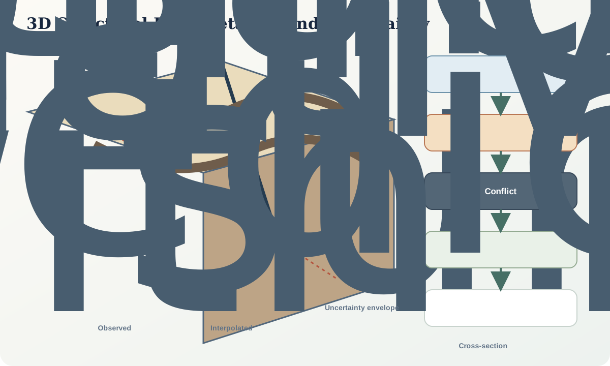
Learning objectives
After this lesson, you should be able to define observations, geological rules and interpolation separately; build topologically consistent fault and fold surfaces; integrate maps, sections, orientation data and depth control; compare explicit and implicit representations; propagate measurement, conceptual and interpolation uncertainty; evaluate alternative event models; and design a new observation that maximally discriminates between them.
Start with a field problem
A mapped fault trace curves around a fold and is intersected by two boreholes. One borehole records a narrow fault at predicted depth; the other encounters repeated stratigraphy 140 m above the first model. Is the fault curved, duplicated, offset by a younger structure, miscorrelated in core, or incorrectly projected from surface?
A smooth surface can be generated through almost any sparse data. Geological interpretation adds rules about continuity, termination, displacement, stratigraphy and event timing, but those rules are hypotheses. The model must show which geometry is observed, which is calculated by interpolation and where a different conceptual model fits the same evidence.
Core process model
A three-dimensional structural model contains surfaces, volumes, lines and topology. Fault surfaces cut or bound rock volumes; horizons terminate against faults or erosional surfaces; folds deform surfaces; intersections create lines; and displacement changes correspondence across faults. Geometry without topology can produce impossible crossing, gaps or duplicated units.
Explicit modelling represents surfaces with triangulated meshes, splines or parametric patches. Implicit modelling represents a scalar field whose iso-surfaces define contacts or foliations. Both require inputs and constraints. Mesh density or a smooth scalar field does not add observations.
Data types include mapped traces, orientation measurements, borehole contacts, oriented core, seismic or other geophysical interpretations, topography and relative-age relations. Each has positional, orientational, resolution and correlation uncertainty. Convert them into common coordinates and preserve original provenance.
Interpolation estimates geometry between observations under a chosen covariance, smoothness, curvature or structural rule. Extrapolation beyond the convex support is less constrained. Fault displacement and fold shape may require restoration or kinematic algorithms rather than independent surface smoothing.
Uncertainty has several layers:
- measurement uncertainty: location, attitude, depth, picking and analytical error;
- sampling uncertainty: unobserved volume and uneven coverage;
- interpolation uncertainty: parameters and mathematical representation;
- conceptual uncertainty: alternative faults, correlations, event sequences and deformation mechanisms;
- implementation uncertainty: coordinate transformations, software settings, mesh resolution and version.
An ensemble can explore parameter variation within one concept, but conceptual alternatives must be built explicitly. A probability-looking volume is meaningful only if the sampling and prior assumptions are stated.
Evidence and measurement
Begin with a data register. Assign stable identifiers, coordinate reference system, units, acquisition method, quality, uncertainty and owner-independent provenance. Keep interpreted contacts separate from raw logs or images. Validate transformations with known control points and round-trip tests.
Use cross-sections as model queries, not decorative independent drawings. A surface that appears in map, section and 3D must be the same object or be reconciled. Check fault–fault intersections, horizon cutoffs, unit order, thickness and displacement consistency. Mark unconstrained terminations.
Compare predictions with withheld data. Leave out selected borehole contacts or orientations, build the model, then measure misfit when they are restored. Spatially clustered validation points do not test remote extrapolation. Report failure as well as fit.
Worked example
A synthetic area records two deformation events.
Event 1: layered rocks were shortened into a northeast-plunging fold above a low-angle reverse fault. S1 is axial planar, and an early vein set V1 cuts bedding but is folded with it.
Event 2: a steep northwest-striking left-lateral fault cuts the fold, offsets the reverse fault and locally reactivates S1 as a brittle fabric. Late veins V2 fill extensional splays and cut V1.
Model A continues the reverse fault as one gently curved surface beneath both boreholes and gives the younger fault 220 m of left-lateral slip. It fits the surface trace, most attitudes and borehole 1. Borehole 2 encounters repeated stratigraphy 140 m shallower than predicted.
Model B introduces an Event 1 thrust splay truncated and offset by the Event 2 fault. It fits both boreholes and predicts a second cutoff in the eastern section, but the splay has no direct surface exposure and adds complexity. Both models honour the high-confidence map trace and V1/V2 timing. Model A is simpler but conflicts with borehole 2; Model B resolves the conflict through an inferred surface.
Do not choose from smoothness alone. Check core correlation and depth first. Then acquire an oriented depth constraint near the predicted eastern cutoff. Intersecting the splay supports Model B; continuous stratigraphy supports a curved or mispositioned Model A. Record the prediction before acquiring the data.
For each surface, store a confidence class: observed, tightly interpolated, broadly interpolated or extrapolated. Build geometry variants within measurement bounds and calculate the range of cutoff positions and unit volumes. Keep Model A and Model B as separate conceptual ensembles.
Misinterpretations and uncertainty
Do not equate a polished rendering with accuracy. Colour, lighting and dense meshes can hide weak support. Display data locations, uncertainty and alternative surfaces alongside the preferred model.
Do not close gaps by inventing hard contacts. If lithology, age or geophysics do not correlate units, leave the relation unresolved. A topologically valid but geologically wrong model remains wrong.
Avoid double counting interpreted derivatives. A map trace digitised from the same geophysical image as a section pick is not independent evidence. Preserve shared provenance in weighting and validation.
Volumes, depths and distances derived from a structural model inherit conceptual uncertainty. Reporting only numerical interpolation variance understates uncertainty when fault number or correlation can change.
Practical investigation
Build a small 3D model from a map trace, twelve orientation measurements, two sections and three synthetic depth contacts. Reserve one contact and three attitudes for validation. Create a minimum-complexity model and an alternative with an extra fault or fold domain. Check topology, unit order, fault cutoffs and withheld-data misfit.
Perturb locations and attitudes within documented uncertainty and rebuild an ensemble for each concept. Plot envelopes at a target depth and calculate the range of intersection locations. Write a model card containing data versions, coordinate system, rules, parameters, validation, conflicts, alternatives and next test.
Mastery check
- What is the difference between geometry and topology?
- Why does a smooth surface not imply strong evidence?
- Which uncertainty is not captured by parameter perturbation within one model?
- How can withheld data test an interpretation?
- What makes a new observation discriminating rather than merely additional?
Sources and further reading
- Uncertainty in 3-D geological modelling, Wellmann and Caumon, 2018.
- Open-source stochastic geological modelling and inversion, de la Varga, Schaaf and Wellmann, 2019.
- Geologic Map Symbol Standard, consistent representation of observed and inferred structures.